Introduction
The empirical variance is one of the best known statistical measures, and it quantifies the spread within a set of drawn samples. It is given by the following formula
\begin{equation} s^2 = \frac{1}{n-1} \sum_{i=1}^{n} \left( x_i - \bar{x} \right)^2 . \end{equation}Today we are going to set out and find a different formula for exactly this empirical variance — one that, as we will see, does not even mention the mean. I first came across it while thinking about how the sum of many samples of a uniform distribution converges towards the normal distribution, by looking at the whole thing inside a vector space. That is an interesting story in its own right, but today it is going to be about the empirical variance only.
Draws as Vectors
Suppose we have \(n\) draws and we now interpret each of them as a coordinate in a vector space. Every dimension represents one draw, and so every set of samples gets its own unique vector. For example
\begin{equation} \text{draw } (x_1, \dots, x_n) \;\longrightarrow\; \text{vector } \vec{x} = \begin{pmatrix} x_1 \\ \vdots \\ x_n \end{pmatrix} . \end{equation}This may look like a trivial way of putting things, but quite a bit can be derived from it. First of all, the assignment even encodes the order of the samples: swap two draws and you land on a different vector. Furthermore, the direction \((1, \dots, 1)^T\) is a very special one. A vector pointing exactly along it has all coordinates equal, so the closer the draw vector lies to this direction, the more evenly the samples are spread around a common value. It is natural to suspect that this direction has something to do with the mean, that is, with the empirical expected value.
The Mean as a Projection
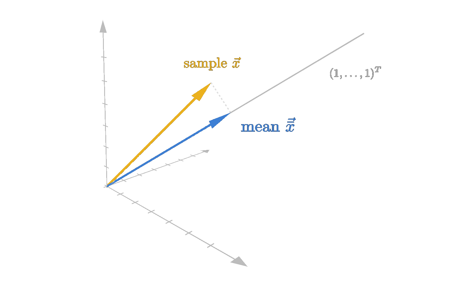
In particular, the mean is then the projection of the draw vector onto the "45 degree direction" \((1, \dots, 1)^T\). Because the scalar product
\begin{equation} \vec{x} \cdot \begin{pmatrix} \frac{1}{n} \\ \vdots \\ \frac{1}{n} \end{pmatrix} = \sum_{i=1}^{n} \frac{x_i}{n} = \frac{1}{n} \sum_{i=1}^{n} x_i = \bar{x} \end{equation}is exactly the mean. There is one blemish to it, though: unfortunately the vector \(\left( \frac{1}{n}, \dots, \frac{1}{n} \right)^T\) does not have length 1, but length \(\frac{1}{\sqrt{n}}\). So geometrically this scalar product is not quite the projection, but the projection times \(\frac{1}{\sqrt{n}}\). It would be preferable to take the vector \(\left( \frac{1}{\sqrt{n}}, \dots, \frac{1}{\sqrt{n}} \right)^T\) instead. Then the scalar product would be exactly the projection, since this one is the unit vector in the "45 degree direction" (let us call it the \(\mu\)-direction).
However, we then end up with
\begin{equation} \vec{x} \cdot \begin{pmatrix} \frac{1}{\sqrt{n}} \\ \vdots \\ \frac{1}{\sqrt{n}} \end{pmatrix} = \frac{1}{\sqrt{n}} \sum_{i=1}^{n} x_i = \sqrt{n}\, \bar{x} \end{equation}at \(\sqrt{n}\) times the actual mean. But! Where exactly does that put us along the \(\mu\)-direction, if we walk this projected length in that direction? It turns out that we land exactly on the vector \(\vec{\bar{x}} := (\bar{x}, \dots, \bar{x})^T\), the vector that carries the mean in every coordinate — because this one has exactly the length
\begin{equation} \left\| \vec{\bar{x}} \right\|_2 = \sqrt{\bar{x}^2 + \dots + \bar{x}^2} = \sqrt{n \bar{x}^2} = \sqrt{n}\, \bar{x} . \end{equation}So projecting the draw vector onto the \(\mu\)-direction does not merely produce a number related to the mean — it lands on the "all coordinates equal" vector that belongs to it. This is a nice geometric interpretation of the mean, and it is something we can actually have a look at visually in 3-dimensional space. One can see nicely how the influence of a single coordinate carries over into the projection, and also that this effect of course decreases as the number of dimensions, i.e. the number of draws, is increased, namely with the square root of \(n\).
The Variance as a Perpendicular Distance
The next question that naturally arises now is: what about the variance? The mean turned out to be the part of the draw vector along the \(\mu\)-direction — so is the variance perhaps the part that is left over, the perpendicular distance to the \(\mu\)-direction?
Well, almost. The perpendicular part of \(\vec{x}\) is the vector \(\vec{s} := \vec{x} - \vec{\bar{x}}\), pointing from the projection to the draw vector itself, and its squared length
\begin{equation} \left\| \vec{s} \right\|_2^2 = \left\| \vec{x} - \vec{\bar{x}} \right\|_2^2 = \sum_{i=1}^{n} \left( x_i - \bar{x} \right)^2 \end{equation}would already be right up to the factor \(1/(n-1)\). But I could of course also compute this squared length via the cross product (as long as we stay in three dimensions for now), right? The cross product gives the area of the parallelogram spanned by \(\vec{x}\) and \(\vec{\bar{x}}\), and area divided by base is height — which is exactly our perpendicular distance.
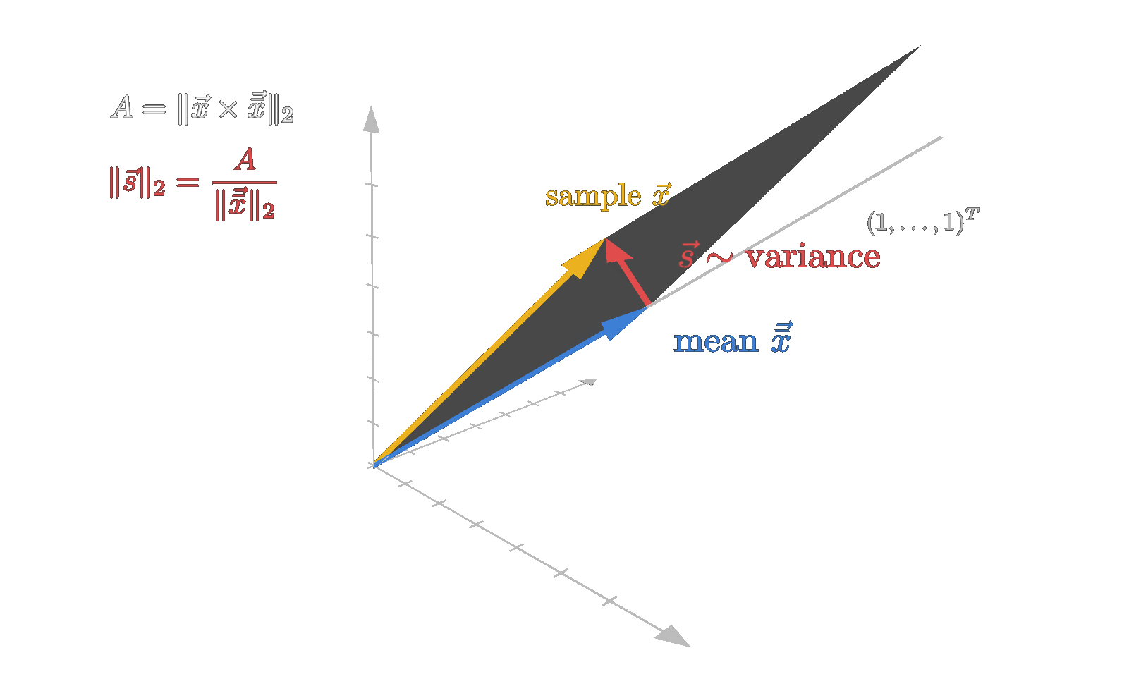
So let us do exactly that:
\begin{equation} \frac{\left\| \vec{x} \times \vec{\bar{x}} \right\|_2^2}{\left\| \vec{\bar{x}} \right\|_2^2} = \left\| \vec{s} \right\|_2^2 = \sum_{i=1}^{n} \left( x_i - \bar{x} \right)^2 . \end{equation}If we now bring in the factor \(1/(n-1)\), we should obtain the empirical variance on the left hand side as well:
\begin{equation} \begin{split} \frac{\left\| \vec{x} \times \vec{\bar{x}} \right\|_2^2}{(n-1) \left\| \vec{\bar{x}} \right\|_2^2} &= \frac{(x_2\bar{x} - x_3\bar{x})^2 + (x_3\bar{x} - x_1\bar{x})^2 + (x_1\bar{x} - x_2\bar{x})^2}{(n-1)\, n \bar{x}^2} \\[6pt] &= \frac{(x_2 - x_3)^2 + (x_3 - x_1)^2 + (x_1 - x_2)^2}{n(n-1)} , \end{split} \end{equation}and something remarkable has happened along the way: the \(\bar{x}\) has cancelled out completely. What remains is a formula for the variance in which no mean appears at all — only the samples themselves. Very interesting — so the variance can also be determined simply by adding up all the squared differences between the samples and then dividing by \(n(n-1)\)?
Before we check that, we first have to generalize the whole thing to arbitrary dimension, because so far the cross product has locked us into \(n = 3\). The generalization of the cross product is the outer product (also called the wedge or exterior product), which collects exactly the same kind of terms, one for every pair of coordinates:
\begin{equation} \left( \vec{u} \wedge \vec{v} \right)_{ij} = u_i v_j - u_j v_i , \quad 1 \leq i < j \leq n , \qquad \left\| \vec{u} \wedge \vec{v} \right\|_2^2 = \sum_{i < j}^{n} \left( u_i v_j - u_j v_i \right)^2 . \end{equation}In the general case we therefore obtain
\begin{equation} \frac{\left\| \vec{x} \wedge \vec{\bar{x}} \right\|_2^2}{(n-1) \left\| \vec{\bar{x}} \right\|_2^2} = \frac{\sum_{i < j} \left( x_i \bar{x} - x_j \bar{x} \right)^2}{(n-1)\, n \bar{x}^2} = \frac{1}{n(n-1)} \sum_{i < j}^{n} \left( x_i - x_j \right)^2 = s^2 . \end{equation}As is easy to follow, we arrive at the same result here as well. All the squared differences between the values simply have to be added up (and then normalised by dividing by \(n(n-1)\)).
Let us have a look at a concrete example. Take the values 3, 5, 6. With the new formula we only need the pairwise differences:
\begin{equation} s^2 = \frac{(3-5)^2 + (3-6)^2 + (5-6)^2}{n(n-1)} = \frac{4 + 9 + 1}{3 \cdot 2} = \frac{14}{6} = \frac{7}{3} \approx 2.33 . \end{equation}With the conventional formula we first need the mean and then the deviations from it:
\begin{equation} \begin{aligned} \bar{x} &= \frac{3 + 5 + 6}{3} = \frac{14}{3} \approx 4.67 , \\[4pt] s^2 &= \frac{1}{n-1} \sum_{i=1}^{n} \left( x_i - \bar{x} \right)^2 = \frac{1}{2} \left[ \left( 3 - \tfrac{14}{3} \right)^2 + \left( 5 - \tfrac{14}{3} \right)^2 + \left( 6 - \tfrac{14}{3} \right)^2 \right] \\[4pt] &= \frac{1}{2} \left[ \left( -\tfrac{5}{3} \right)^2 + \left( \tfrac{1}{3} \right)^2 + \left( \tfrac{4}{3} \right)^2 \right] = \frac{1}{2} \left[ \frac{25}{9} + \frac{1}{9} + \frac{16}{9} \right] = \frac{1}{2} \cdot \frac{42}{9} = \frac{7}{3} \approx 2.33 . \end{aligned} \end{equation}Both ways give the same value, as expected — but notice how differently they get there: the pairwise route never leaves the integers until the final division, while the conventional route drags thirds and ninths through every single step.
Is This Actually Better?
Is our new formula actually more efficient? Well, that depends on \(n\). For very small \(n \leq 5\) it indeed is. Beyond that it becomes very inefficient very quickly, since the number of differences grows quadratically with \(n\): there are \(\binom{n}{2} = \frac{n(n-1)}{2}\) pairs, whereas the conventional formula only needs a number of operations that grows linearly with \(n\).
But the formula holds a completely different advantage, the one we just saw in the example. If the given values are integers, then integers are preserved throughout the computation as well. In this case the variance can be computed in one's head far more easily, and the result can be written down as a fraction straight away. The only exception would be if one wants to write that fraction out as a decimal number. But even this is just a single division that can often be carried out quickly in one's head.
Compare that to the conventional formula: first the mean has to be computed, which is usually already a decimal number, then the differences to the individual values, which are then again decimal numbers, and finally these decimal numbers have to be squared, summed, and divided by \(n-1\). In one's head that is practically impossible.
Lagrange Identity
But what is this actually, this thing we have ventured into here? Well, in principle we have simply used the outer product to transform the sum formula for the variance into a different summation. We took this route via a geometric insight and, along the way, also found some nice geometric intuitions for the mean and the variance in a vector space. But put simply, the core of the whole thing is nothing other than the Lagrange identity applied to the sum formula of the variance.
The Lagrange identity describes exactly this possible transformation, one that can always be applied to any such sum. It is closely tied to vector spaces and the outer product, and it is defined as follows:
\begin{equation} \left( \sum_{i=1}^{n} a_i^2 \right) \left( \sum_{i=1}^{n} b_i^2 \right) - \left( \sum_{i=1}^{n} a_i b_i \right)^2 = \sum_{i<j}^{n} \left( a_i b_j - a_j b_i \right)^2 . \end{equation}In a vector space it can also be written down in a simplified way as
\begin{equation} \left\| \vec{a} \right\|_2^2 \left\| \vec{b} \right\|_2^2 - \langle \vec{a}, \vec{b} \rangle^2 = \left\| \vec{a} \wedge \vec{b} \right\|_2^2 . \end{equation}And this is exactly what we did, without calling it by its name: with \(\vec{a} = \vec{x}\) and \(\vec{b} = \vec{\bar{x}}\), the left hand side is the squared area of the parallelogram spanned by the two vectors, and dividing by \(\left\| \vec{\bar{x}} \right\|_2^2\) leaves exactly the squared perpendicular distance to the \(\mu\)-direction. So our "cross product trick" was never a trick of three dimensions — it is this identity, and it works in every dimension.
Conclusion
So what did we end up with? We started with the well-known formula for the empirical variance, took the samples seriously as coordinates of a single vector, and found that the mean is a projection onto the "45 degree direction" and the information of the variance is in the perpendicular distance to it. Following that picture led us to a formula that needs no mean at all: add up all squared differences between the samples and divide by \(n(n-1)\). In the end this turned out to be not a new theorem but the Lagrange identity in disguise — and honestly, I find that the nicer outcome - we got a beautiful geometric explanation for why two long-known formulas have to agree.
And the pairwise view is worth keeping in mind anyway. For small samples it is genuinely the fastest way to compute the variance in your head, since with integer values everything stays an integer until the very last division. And it tells you what the variance is without ever mentioning the mean: half the average squared difference between two draws. Sometimes it just pays off to take a formula you have seen a hundred times and look at it from a direction it was never meant to be looked at from.