Introduction
To understand the derivation of the distribution of the sample mean of a normally distributed sample, it is important to become familiar with the concept of applying a function to a random variable, particularly to a normally distributed one. We will not go into the details of this prerequisite so if needed make sure you have read the according Stories about this topic.
Looking at the sample mean and interpreting it as a new random variable yielded by a function of random variables we see that it is simply a sum scaled by a factor
\begin{equation} Y = \frac{1}{n} \sum_{i=1}^n X_i \quad X_i \sim \mathcal{N}(\mu,\sigma^2). \end{equation}Using the standard approach to solve for the distribution of \(Y\), that is examining the cumulative probability, we obtain
\begin{equation} P(Y \leq y) = P(\frac{1}{n} \sum_{i=1}^n X_i\leq y), y \in \mathbb{R}. \end{equation}The next step is to isolate the \(X_i\) since we already know their distribution. However, this does not appear to be possible in this case. Of course, we could multiply by \(n\) to eliminate the scaling factor but then we are kind of stuck. Nevertheless, we can resolve this by interpreting the above equation in a geometric context.
Geometrical perspective on the sample mean
Let us switch from the cumulative probability to the density and consider what this sum actually represents. Imagine the vector space where each \(X_i\) corresponds to a coordinate axis and a specific point in that space represents a single sample \((x_i,\cdots,x_n)\) that we have drawn. The sum \(\sum_{i=1}^n X_i\) then defines a hyperplane (compare \(x_1 + x_2 + x_3 = 2\) for a plane in 3 dimensions). In other words, if we examine the probability density function \(PDF_Y(y)\) at a specific value \(y\), we are considering the probability
\begin{equation} P(Y = y) = P\Big(\frac{1}{n} \sum_{i=1}^n X_i = y\Big). \end{equation}We realize that all possible samples \(x_i\) that yield the same \(y\) lie on the same hyperplane. Let us clarify this by looking at a graphical representation. The following figure illustrates this for the 3-dimensional case.
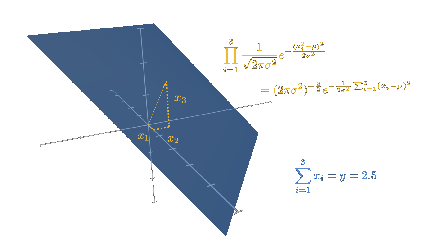
As can be deduced from the illustration above, the set of all \(x_i\) that sum to a constant \(y\) forms a plane. For each specific constant \(y\), there is a corresponding plane.
Realizing that we now should be able to find a formula for the density of \(Y\). The density is essentially just about how often a random variable is equal to some constant. In our case a constant \(y\) defines a hyperplane, so we can just integrate the probabilities of all samples \((x_1,\cdots,x_n)\) that lie on that plane. Since the \(x_i\) are independent, the probability of a single point \((x_1,\cdots,x_n)\) in this space (representing the drawn sample) can be expressed as the product of the probabilities of each \(x_i\). And since all \(x_i\) follow the same normal distribution this leads to
\begin{equation} P(X) = \prod_{i=1}^n \frac{1}{\sqrt{2\pi\sigma^2}}e^{(x_i-\mu)^2 / 2 \sigma^2} \end{equation} \begin{equation} = (2\pi\sigma^2)^{-\frac{n}{2}}e^{\sum_{i=1}^n\frac{(x_i-\mu)^2}{2 \sigma^2}}. \end{equation}Integrating the above probability over the specific plane given by the constant \(y\), gives us
\begin{equation} Y_{PDF}(y) = \int_{\text{plane}} (2\pi\sigma^2)^{-\frac{n}{2}}e^{\sum_{i=1}^n\frac{(x_i-\mu)^2}{2 \sigma^2}} dx_1.. dx_n. \end{equation}Now, the question is of course how to we solve this integral? It is not a trivial task. However, you might already know, or you may realize by considering the sum of squares, that the function we are integrating, a multivariate normal distribution, is rotationally symmetrical. That means the integral is invariant under rotations about the origin. Therefore, without loss of generality, we can assume that the plane is normal to one of the axes, which, in equation form, can be expressed as \(x_j = \text{const}\). Specifically, we can choose the plane \(x_n = \text{const}\), which is normal to the last axis.
The remaining question is, what is the constant in our rotated plane \(x_n = \text{const}\) if the original plane was described by the sum being equal to \(y\)? Since a rotation about the origin does not change the shortest distance from the plane to the origin, the constant in \(x_n = \text{const}\) will simply be this minimal distance to the origin. Because when the plane is aligned such that it is normal to one axis the minimal distance to the origin is obviously exactly along that axis.
But how can we determine this minimal distance? Since the equation represents an unweighted sum, the original unrotated plane is normal to the vector direction \((1,1,\cdots,1)\). Therefore, the minimal distance to the origin is the length from the origin to the plane along this direction. The following illustration helps clarify this concept.
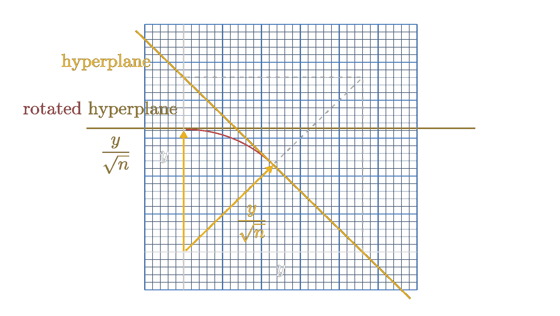
Above, the situation is shown for the 2-dimensional case. We see that we can easily calculate this distance using the pythagoras, which yields
\begin{equation} const. = d_{\text{minimal}} = \frac{\sqrt{y^2 + y^2}}{2} = \frac{y}{\sqrt{2}}. \end{equation}Obviously, if we generalize to \(n\) dimensions, we see that
\begin{equation} const. = d_{\text{minimal}} = \frac{\sqrt{n y^2}}{n} = \frac{y}{\sqrt{n}}. \end{equation}If you do not see this generalization immediately, you can just intersect the plane with the direction vector \((1,1,\cdots,1)\), which will yield the vector of intersection to be \(\frac{1}{n}\) times the direction vector and the length of this vector intersection obviously evaluates to \(\frac{1}{\sqrt{n}}\).
Now, let us come back to the integral we tried to solve. We now know that we have to integrate along the plane given by \(x_n = \text{const.} = \frac{y}{\sqrt{n}}\). With this in mind, we can see that it reduces to
\begin{equation} Y_{PDF}(y)dy = \frac{1}{\sqrt{2\pi\sigma^2}}e^{(x_n-\mu)^2/ 2 \sigma^2} \end{equation} \begin{equation} \cdot \int_{\text{plane}} (2\pi\sigma^2)^{-\frac{n-1}{2}}e^{\sum_{i=1}^{n-1}(x_i-\mu)^2/ 2 \sigma^2} dx_1.. dx_{n-1}, \end{equation}where we have moved the normal distribution of the \(n^{\text{th}}\)-axis outside the integral because it is constant with respect to the integral over the plane. This is a direct consequence of defining the plane with \(x_n = \text{const.}\).
We are now left with an integral over the entire space along the plane of probability density functions of a normal distribution. Regardless of the specific distribution, these always evaluate to 1, as that is how a probability density function (PDF) is defined. Hence, we are left with
\begin{equation} Y_{PDF}(y)dy = \frac{1}{\sqrt{2\pi\sigma^2}}e^{(x_n-\mu)^2/ 2 \sigma^2}. \end{equation}Using the fact that \(x_n=\frac{y}{\sqrt{n}}\) and applying this change of variables (note: \(dx_n = -\frac{1}{\sqrt{n}dy}\)) we are able to obtain the solution for the \(PDF\) of \(Y\)
\begin{equation} Y_{PDF}(y)dy = \frac{1}{\sqrt{2\pi n\sigma^2}}e^{\frac{(y-\mu)^2}{2 n\sigma^2}}dy = \mathcal{N(0,n\sigma^2)}. \end{equation}Remember we simplified \(Y\) to be only the summation omitting the scale factor \(\frac{1}{n}\). However, a scale factor applied to a normal distribution is pretty trivial, it is again a normal distribution just with the variance scaled by that factor. We already showed this in this Story. Including the scale factor let us arrive at the final solution
\begin{equation} \bar{X}_{PDF}(x) = \frac{\sqrt{n}}{\sqrt{2\pi \sigma^2}}e^{nx^2/ 2 \sigma^2}dy = \mathcal{N(0,\frac{\sigma^2}{n})}. \end{equation}And there we have it, the distribution of the sample mean of a normally distributed sample, which is again a normal distribution but with a reduced variance. The extent of this reduction depends on the number of samples \(n\). Intuitively, this also makes sense because, with more samples, we expect the sample mean to more accurately reflect the true mean\(\mu\).
Sample size
To conclude this Story, let us examine how the distribution behaves with different sample sizes. In particular, let us explore how quickly this distribution converges to a spike at the true mean. Essentially, we want to determine how many samples are needed to confidently assert that the sample mean is very close to the true mean.
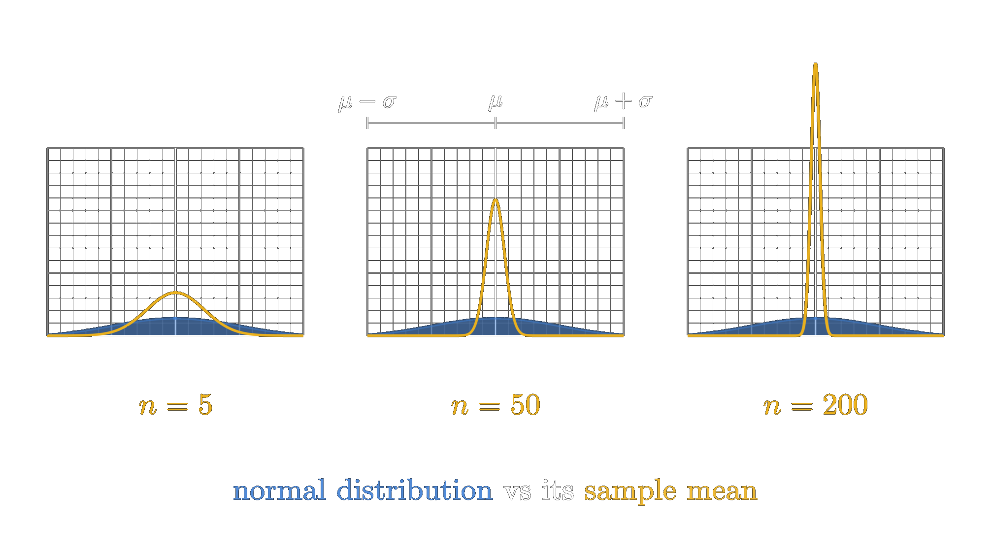
In the illustration above the sample mean distribution for three different sample sizes of 5, 50, and 200 is shown in yellow. The red curve in the background is the original normal distribution from which the samples have been drawn. The graphs are standardized, such that the left edge is exactly one standard deviation \(\sigma\) lower than the mean \(\mu\) and the right edge one standard deviation higher.
We observe that with a very small number of samples, the distribution of the sample mean remains quite similar to the original distribution, maintaining a similar deviation from the mean \(\mu\). However, as the sample size increases to 50, the distribution of the sample mean begins to show a distinct peak at the true mean \(\mu\). The probability that the sample mean significantly overestimates or underestimates \(\mu\) becomes very close to zero. As the number of samples continues to increase, this trend becomes even more pronounced, with the peak at the true mean becoming sharper.
Therefore, we can conclude that, with sufficiently large sample sizes, the sample mean becomes quite accurate, and the error made by assuming this sample mean equals the true mean becomes very small. However, it is important to note that the standard deviation of the sample mean distribution decreases at a rate proportional to \(\frac{1}{\sqrt{n}}\). This means that to halve the standard deviation, the number of samples must be quadrupled. This is a crucial consideration when working with sample means.
With this remark, we will conclude this Story. We have seen that the sample mean of a normally distributed sample also follows a normal distribution, with a variance that decreases as the number of samples increases. This highlights a fundamental principle in statistics: larger sample sizes lead to more reliable estimates of the population mean, but needless to say with increasing expenses in gathering those samples.