Introduction
Yeah, about those Stirling numbers. When you start to play around with difference equations like Stirling did back in the day, you will soon notice that if you are looking for a solution of those, it makes a lot of sense not to use the standard power basis, like
\begin{equation} T(z) = a_0 + a_1 z + a_2 z^2 + a_3 z^3 + \dots , \end{equation}but to slightly deviate from it and use falling powers as your basis, like
\begin{equation} T(z) = b_0 + b_1 z^{\underline{1}} + b_2 z^{\underline{2}} + b_3 z^{\underline{3}} + \dots , \qquad \text{where} \qquad z^{\underline{k}} = z (z-1) (z-2) \cdots (z-k+1) . \end{equation}And when you then investigate how to transform between those two bases, you will soon find a particular structure in the coefficients — namely the Stirling numbers:
| 1 | 1 | 1 | 1 | 1 | 1 |
| 1 | 3 | 7 | 15 | 31 | |
| 1 | 6 | 25 | 90 | ||
| 1 | 10 | 65 | |||
| 1 | 15 | ||||
| 1 |
Here shown are only those of the second kind, as they will be the focus of this Story.
Also, Stirling numbers are a lot about brute forcing your way through problems by calculating chances the no-replacement way, when the problem actually would require you to use the with-replacement approach. Because if you know the Stirling numbers, you can do just that. It would not make a lot of sense though, because the with-replacement one is just a simple power expression. However, it is this shift between those two perspectives that is, in some sense, the essence of the Stirling numbers.
But anyway, let's start from the very beginning — and by the very beginning I mean the very beginning. So let's open the Methodus Differentialis, Stirling's famous work from the year 1730, and have a detailed look at how he arrived at this special kind of numbers. After that we are going to see how one would arrive at these numbers in general and what they are actually about. In some sense they are just another kind of binomial coefficient, counting the possibilities of a certain combinatorial problem — but of course those things pop up all over the place, and the main place for the Stirling numbers is discrete calculus, especially difference equations. But now let's really get started and look at the relevant pages of Stirling's work.
Series, Sequences and Difference Equations
First, Stirling describes how a series (or a sequence — the two notions often blur into each other in Stirling's writing) such as, for example,
\begin{equation} 1, \; 3, \; 9, \; 27, \; 81, \; \dots \end{equation}can be described by a difference equation. For this he denotes the individual terms by \(T\), \(T^{I}\), \(T^{II}\), and so on, and the position of a term he calls \(z\).
In the series above, for instance, it is easy to see that every further term is reached by continued multiplication by \(3\), that is
\begin{equation} T^{I} = 3\, T . \end{equation}So this one relation can be written down as a general expression, valid at every position \(z\). This is a so-called difference equation. If one additionally has an initial value — here \(T = 1\) at \(z = 0\) — the series, or sequence, is uniquely defined by it.
The whole thing can also be seen as the discrete analogue of a differential equation. And just as with those, the question of a solution of these equations comes up. So suppose a difference equation is given, say something of the form
\begin{equation} T^{I} = f(z)\, T \qquad \text{or, more generally,} \qquad F\!\left( z, \, T, \, T^{I}, \, T^{II}, \dots \right) = 0 . \end{equation}How does one then get to a general expression \(T(z)\), from which the individual terms of the series, or members of the sequence, can be determined directly?
There are all kinds of ways to get there: guessing a solution and verifying it, the characteristic equation for linear equations with constant coefficients, telescoping, generating functions, or — in modern language — the z-transform. Stirling, probably because with what he dealt with were mostly power series anyway, takes the ansatz of simply writing the solution as a power series with unknown coefficients, and then solving the system of equations that the difference equation induces on them.
Solving a Difference Equation via a Power Series
Let us watch this ansatz at work on a concrete equation. Take
\begin{equation} T^{I} - T = z^2 , \qquad T = 0 \; \text{at} \; z = 0 , \end{equation}which is nothing exotic: it says that the terms grow by the squares, so \(T(z)\) is simply the sum of the first squares, \(T(z) = 0^2 + 1^2 + \dots + (z-1)^2\) — finding closed forms for sums of this kind is exactly the sort of problem the Methodus Differentialis is concerned with. Following Stirling, we make the ansatz of a power series with unknown coefficients:
\begin{equation} T(z) = a_0 + a_1 z + a_2 z^2 + a_3 z^3 + a_4 z^4 + \dots \end{equation}What we are given is the difference equation, so we have to see what the difference \(T(z+1)-T(z)\) means when we consider \(T\) to be a power series. Doing that yields
\begin{equation} T^{I} - T = \sum_{k=1}^{\infty} a_k \left( (z+1)^k - z^k \right) , \end{equation}we see already that \(a_0\) vanishes completely, so this value can be chosen arbitrarily. This directly corresponds to the integration constant in the continuous case. So, this \(a_0\) will be chosen to meet the initial value we are given, our boundary condition.
For the rest of the coefficients, we see that we receive a binomial expression where the highest power \(z^k\) is cut off. So let us start to write out the first few differences
| \(a_1\) | \(1\) |
| \(a_2\) | \(2z+1\) |
| \(a_3\) | \(3z^2+3z+1\) |
| \(a_4\) | \(4z^3+6z^2+4z+1\) |
| \(a_5\) | \(5z^4+10z^3+10z^2+5z+1\) |
Here we already see the first problem that arises: All the differences have also terms of lower powers in \(z\). So even the coefficient \(a_{1000}\) will affect the term of \(z^2\) or \(z\).
But let us make a small assumption here. Because we know this difference power series has to evaluate to \(z^2\) - and that we have already covered when we reach the term \(a_3\). So it is definitely possible to construct a solution if we cut our series here and set all the other coefficients \(a_k = 0 \text{ if } k>3\). What survives of our infinite ansatz is then,
\begin{equation} T^{I} - T = a_3 \left( (z+1)^3 - z^3 \right) + a_2 \left( (z+1)^2 - z^2 \right) + a_1 = 3 a_3 \, z^2 + \left( 3 a_3 + 2 a_2 \right) z + \left( a_3 + a_2 + a_1 \right) . \end{equation}Comparing this finite set of coefficients with \(z^2\) gives us then also a finite system of equations: \(3 a_3 = 1\), then \(3 a_3 + 2 a_2 = 0\), then \(a_3 + a_2 + a_1 = 0\), and the initial value forces the arbitrary constant \(a_0\) to be \(0\). Solving the equation system from the top down yields \(a_3 = \frac{1}{3}\), \(a_2 = -\frac{1}{2}\), \(a_1 = \frac{1}{6}\), so for the final result we get
\begin{equation} T(z) = \frac{z^3}{3} - \frac{z^2}{2} + \frac{z}{6} = \frac{z(z-1)(2z-1)}{6} . \end{equation}That works, and it will always work — but notice where the labour went. All of it was spent expanding \((z+1)^k\) with the binomial theorem and untangling how the powers mix into each other. We had to sneak in a little justification to not end up with an endless system of equations. So we already see, the basis \(1, z, z^2, z^3\) simply does not get along with the operation "step one position forward" very well. Ideally we want to change the ansatz a little bit such that the powers of \(z\) are more isolated regarding the coefficients \(a_k\).
So let us have a look at how something like this can be achieved. Write the difference of consecutive terms as its own operator, \(\Delta T = T^{I} - T\) — essentially the discrete counterpart of the derivative. When we try to use falling powers so \(z(z-1)(z-2)\dots\) as a basis for this operator we get:
\begin{equation} \Delta \, z^{\underline{k}} = (z+1) z \cdots (z-k+2) - z (z-1) \cdots (z-k+1) = z^{\underline{k-1}} \left( (z+1) - (z-k+1) \right) = k \, z^{\underline{k-1}} . \end{equation}So considering the difference of a falling power \(z^{\underline{k}}\) is just \(k\) times the falling power of \(k-1\). That is a perfectly clean result and differences of higher powers will no longer smear into the lower powers. Essentially it is precisely like the power rule \(\left( x^k \right)' = k x^{k-1}\) for the continuous case, only with falling powers in place of powers. So in this basis, solving \(\Delta T = z^2\) is mere antidifferentiation. Convert the right hand side once,
\begin{equation} z^2 = z(z-1) + z = z^{\underline{2}} + z^{\underline{1}} , \end{equation}and read off the solution term by term, just as one would integrate a polynomial:
\begin{equation} T(z) = \frac{z^{\underline{3}}}{3} + \frac{z^{\underline{2}}}{2} = \frac{z(z-1)(z-2)}{3} + \frac{z(z-1)}{2} = \frac{z(z-1)(2z-1)}{6} . \end{equation}Same result, no binomial expansion, no system of equations — the only real work left is the conversion of \(z^2\) into falling powers. And the coefficients showing up in that conversion, the \(1\) and \(1\) in front of \(z^{\underline{2}}\) and \(z^{\underline{1}}\)? Those are Stirling numbers of the second kind. The entire difficulty of difference equations has been pushed into one translation table between the two bases — and that table is what this story is about.
Transforming Between the Two Bases
Now we have seen how powerful this idea of a falling power series is regarding difference equations. The main task for solving difference equations is then just knowing how to transform from the standard basis of powers of \(z\) (because this is the form most difference equations will be given in) to the falling power basis. And of course also to transform the found solution back to powers of \(z\) (if one prefers to write it in the conventional way again).
Therefore Stirling investigates exactly this. Right at the start of the Methodus, he sets up the representation of a power in terms of falling powers,
\begin{equation} z^m = c_1 \, z^{\underline{1}} + c_2 \, z^{\underline{2}} + \dots + c_m \, z^{\underline{m}} , \end{equation}and asks for the coefficients \(c_k\) — and the columns of the table at the very top of this post are nothing else than these coefficients, one column per power. So how do you get them? By doing to \(z^m\) exactly what the falling powers themselves suggest: peel off the factors \(z\), \((z-1)\), \((z-2)\), … one after the other, by repeated division. The remainder that falls off at each stage is one coefficient. Let us do it for \(z^3\). Pulling out the factor \(z\) is free,
\begin{equation} z^3 = z \cdot z^2 . \end{equation}Now divide the remaining \(z^2\) by \((z-1)\), which leaves remainder \(1\),
\begin{equation} z^2 = (z-1)(z+1) + 1 \qquad \Longrightarrow \qquad z^3 = z(z-1)(z+1) + z , \end{equation}and there the first coefficient has fallen off: \(c_1 = 1\), sitting in front of \(z^{\underline{1}} = z\). Next, divide the remaining \((z+1)\) by \((z-2)\), which leaves remainder \(3\),
\begin{equation} z + 1 = (z-2) + 3 \qquad \Longrightarrow \qquad z^3 = z(z-1)(z-2) + 3\, z(z-1) + z , \end{equation}and we are done:
\begin{equation} z^3 = z^{\underline{3}} + 3 \, z^{\underline{2}} + z^{\underline{1}} . \end{equation}There they are — the \(1\), \(3\), \(1\) of the third column of the table. Every column can be computed like this: keep dividing by the next factor \((z-k)\) and collect the remainders. This is essentially what Stirling does; in Ian Tweddle's annotated translation of the Methodus, his computation of the table is laid out in detail.
Funnily enough, there would have been a shortcut available. Each power is just \(z\) times the previous one, \(z^{m+1} = z \cdot z^m\), and multiplying a falling power by \(z\) is a one-liner: since \(z = (z-k) + k\),
\begin{equation} z \cdot z^{\underline{k}} = (z-k) \, z^{\underline{k}} + k \, z^{\underline{k}} = z^{\underline{k+1}} + k \, z^{\underline{k}} . \end{equation}So every entry of a new column is obtained from the previous column as \(c_k^{(m+1)} = c_{k-1}^{(m)} + k \, c_k^{(m)}\) — take the entry diagonally above, add \(k\) times the entry directly to the left, done.
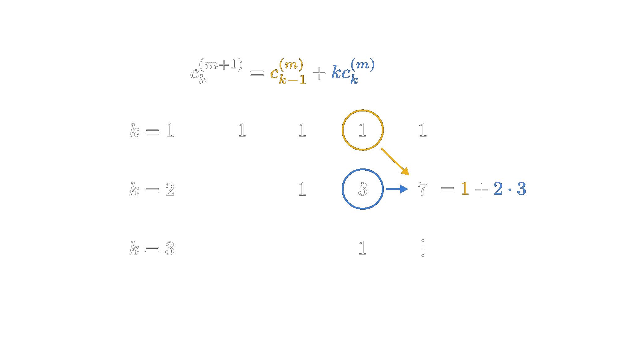
That is how one would fill in the table today, column by column, without a single division. Stirling, as Tweddle remarks in his annotations, apparently did not know this recurrence — his table, computed the laborious way, is correct all the same.
This is how you get the Stirling numbers — of the second kind, to be precise. But what about those of the first kind then? Well, those are just the numbers that arise when you want to transform the other way round. So if you are given an expression in falling powers and you want to convert it into an expression in standard powers.
Obviously, they are heavily related to the Stirling numbers of the second kind, but they are still actually about something slightly different. And also, in order to keep this story short and clear, I want to skip them here and have a separate detailed look at them in another story.
By the way, the reason I went with the second kind first is to keep the order in which Stirling presented them in his publication
Let us look at a concrete expression and see how one would use the Stirling numbers in practice. Since the transformation is linear, there is nothing new to learn: every power gets converted separately — each one is exactly one column of the table — and afterwards we collect. Take, for instance,
\begin{equation} z^4 + 2 z^3 - 11 z^2 - 12 z . \end{equation}Reading off the first four columns of the table gives
\begin{equation} \begin{aligned} z^4 &= z^{\underline{4}} + 6 \, z^{\underline{3}} + 7 \, z^{\underline{2}} + z^{\underline{1}} , \\ z^3 &= z^{\underline{3}} + 3 \, z^{\underline{2}} + z^{\underline{1}} , \\ z^2 &= z^{\underline{2}} + z^{\underline{1}} , \\ z &= z^{\underline{1}} . \end{aligned} \end{equation}Now multiply each line by its coefficient from the expression and add everything up, falling power by falling power:
\begin{equation} z^4 + 2 z^3 - 11 z^2 - 12 z = z^{\underline{4}} + \left( 6 + 2 \right) z^{\underline{3}} + \left( 7 + 2 \cdot 3 - 11 \right) z^{\underline{2}} + \left( 1 + 2 - 11 - 12 \right) z^{\underline{1}} , \end{equation}and so
\begin{equation} z^4 + 2 z^3 - 11 z^2 - 12 z = z^{\underline{4}} + 8 \, z^{\underline{3}} + 2 \, z^{\underline{2}} - 20 \, z^{\underline{1}} . \end{equation}No algebra beyond looking up four columns and adding. And once an expression is written in this form, everything from before becomes available again: differences and antidifferences can be read off with the discrete power rule — so, for example, summing this polynomial over the first \(z\) integers is now a one-liner.
A Different Perspective
But let us now look at the whole thing from a different perspective. To see the full picture what the Stirling numbers are actually about in the broader context.
In principle we have the following problem: we want to know how to represent a power \(z^n\) through falling factorials,
\begin{equation} z^n = \sum_{k=0}^{n} a_k \, z^{\underline{k}} . \end{equation}The coefficients appearing in it are the Stirling numbers (the second kind to be precise), as we have already seen above — they let us transform into the basis of falling factorials.
But let us look at the problem statement once more, this time without knowing the \(a_k\) already. How could we solve this problem? What are powers actually, and where do falling factorials show up?
A power can stand for the volume of an \(n\)-dimensional cube — or for probabilities and possibilities: for example, when I select from \(z\) things \(n\) times.
Falling factorials likewise describe an \(n\)-dimensional volume (every multiplication can always be interpreted that way), but the more natural reading here is again the counting of probabilities and possibilities. Because if I select from \(z\) things \(n\) times but cannot select the same thing twice — without replacement, so to speak — then I inevitably end up with the multiplication \(z(z-1)(z-2)\cdots(z-n+1)\).
So what does the equation
\begin{equation} z^n = \sum_{k=0}^{n} a_k \, z^{\underline{k}} \end{equation}actually mean in that sense?
Well, let us picture it with a concrete example. We have 3 circles and want to paint them, with four colours available. How many possibilities are there?
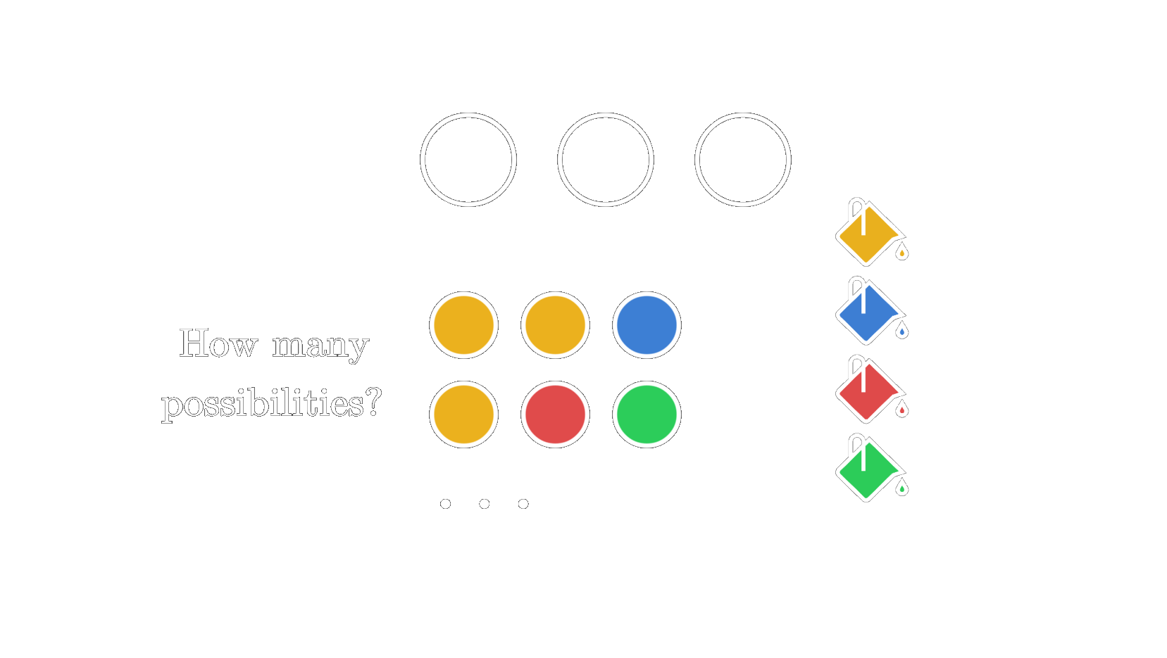
The simple answer is of course: I have 4 possibilities for each circle, so there are \(4^3\) possibilities in total.
However, one could also start by saying there are \(4 \cdot 3 \cdot 2\) possibilities. That only counts the possibilities where the three circles are painted in three different colours — but if we know which other possibilities we have forgotten along the way, and add those up as well, we should still arrive at the correct result in the end, shouldn't we?
What we have forgotten are, for one, all the cases where there are only two distinct colours — two circles sharing the same colour. How many possibilities are there to colour the two blocks of circles in this case? Naturally, 4 colours for the first block and 3 for the second (we are not allowed to pick the same one again — otherwise there would not be two groups, all circles would simply be of one colour). The question, of course, is how many different arrangements there are: the first two circles could be the ones sharing a colour, or the last two, and so on. But let us save that for the end.
We have also forgotten the cases where all three circles have the same colour. Of those there are, consequently, 4 possibilities — one for each colour.
If we now add up all these variants, we should have covered every possibility.
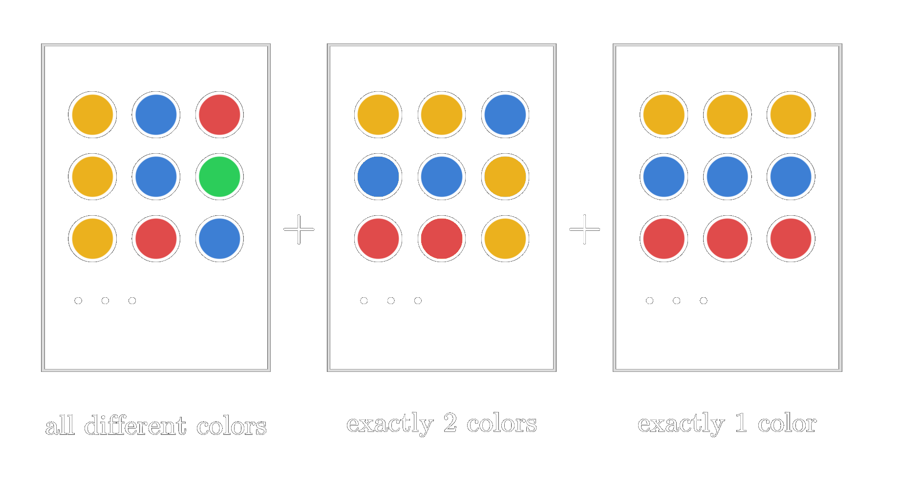
The only question left is how often each variant occurs. The first one — all colours different — and the last one — all colours the same — obviously occur just once. For the one where exactly two are the same, there are three in total: the two on the left, the two on the right, or the two outer ones. So we can now write
\begin{equation} 4^3 = 1 \cdot [4 \cdot 3 \cdot 2] + 3 \cdot [4 \cdot 3] + 1 \cdot [4] . \end{equation}The equation from before corresponds exactly to this split — with \(z = 4\), \(n = 3\), it reads \(4^3 = 1 \cdot 4^{\underline{3}} + 3 \cdot 4^{\underline{2}} + 1 \cdot 4^{\underline{1}}\), and there they are again, the \(1\), \(3\), \(1\) from the third column of the table. The Stirling numbers are exactly this number of variants: how often do I have to take these without-replacement possibilities so that, in total, I end up with all the with-replacement possibilities. And what exactly were these variants?
In how many ways can I form of \(n\) things \(k\) non-empty blocks — in our example the blocks arise from certain circles having the same colors; and that is what the coefficients of the transformation
\begin{equation} z^n = \sum_{k=0}^{n} a_k \, z^{\underline{k}} \end{equation}are (also) about in the end.
Conclusion
I want to make some final remarks regarding our concrete example of colouring the circles. It makes a lot of sense to complicate things a little more and also think this through with 4 circles. Because then the numbers really start to become kinda odd and drift away from the binomial stuff. For example, when you want to collect the case where three circles have the same colour, so only two colours are used, you simultaneously want, of course, the case where two circles are of the same colour and the other two also of one different colour. Because in both cases only 2 colours are used. Evidently, the number of possibilities (if you still use 4 colours) will be \(4 \cdot 3\) for both. But that is how you then get to those kinda weird numbers like the 7. Because in the end it is just about how you can form a certain number of blocks — in this example, how you can form two blocks out of four things. So, the number of partitions of a set into non-empty blocks.
And what about the volume interpretation of \(z^n\) and the factorials? Well, of course, you can also do just that. It then becomes a question of how you can permute the lattice points. The points fall into different classes: those where all three coordinates are equal (since we have 3 circles, this corresponds to all circles having the same colour), those where exactly two coordinates coincide, and so on. You end up with the same count — but it is a genuinely interesting structure once you visualize it. We will not go into the details here; I will simply leave you with this beautiful visualization showing the structure of the Stirling numbers in three dimensions.
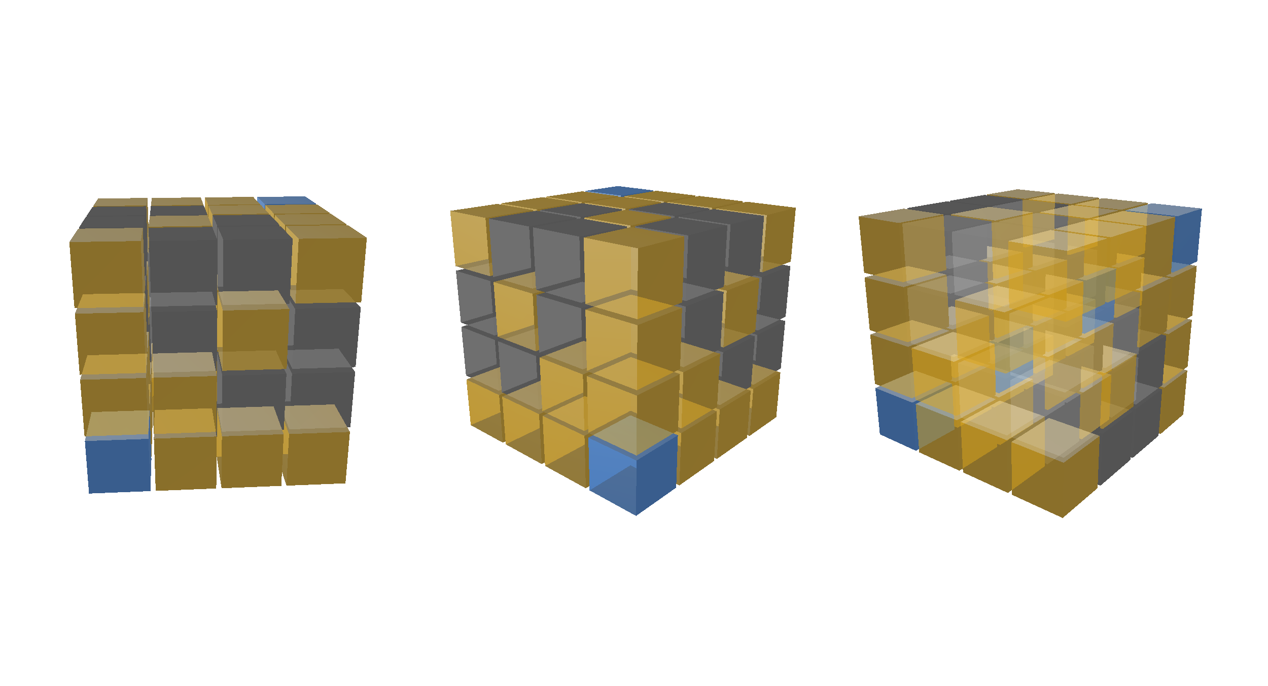
And with that we will conclude this story. We opened a book from 1730 because of some difference equations, noticed that the operation "step one position forward" hates the basis \(1, z, z^2, \dots\) and loves the falling powers, and found that the entire difficulty of moving between the two worlds is compressed into one triangular table. And then that table turned out not to be some arbitrary pile of coefficients at all: its entries count in how many ways \(n\) things can be split into \(k\) non-empty blocks. Which is exactly the shift from the introduction — the with-replacement world, counted through the without-replacement pieces it is made of.
What is still missing is the way back — the Stirling numbers of the first kind, which undo this transformation and bring a combinatorial story of their own along. That one is for another time. Until then: whenever a power and a factorial meet somewhere in discrete mathematics, chances are a Stirling number is standing between them.