Introduction
An interesting question that one quickly stumbles upon is the sum of square numbers. The story of the sum of consecutive integers is relatively well known, as it was Gauss who, already as a young student, discovered a simple closed formula for it. As a brief reminder, this formula can be derived very easily by pairing the \(i\)-th term with the \((n-i)\)-th term.
For example, when summing the numbers from 1 to 100, we pair \(1\) with \(100\), \(2\) with \(99\), and so on. Each of these pairs sums to \(101\), that is, \(n+1\). Since there are exactly \(50\) such pairs (or in general \(n/2\)), the sum of the first \(n\) natural numbers is given by
\begin{equation} S_n = (n+1)\frac{n}{2} \end{equation}But what happens if we consider square numbers instead? In this Story we will take a little explorative walk to arrive at a formula that spits out the sum up to \(n\) square numbers, like Gauss's equation for the consecutive integers.
Summing Squares: Playing with Geometry
Let us begin by writing down the sum we are trying to solve and its first few values of the sequence
\begin{equation} \sum_{i=1}^n i^2 = 1 + 4 + 9 + 16 + \dots \end{equation}The trick of pairing the \(i\)-th term with the \((n-i)\)-th term clearly no longer works here. The pairwise sums are no longer constant. That is actually due to the fact that the sequence of square numbers is curved rather than linear. For example summing up all even numbers, or every third number (like \(1, 4, 7, 10, \dots\) Gauss's trick would actually work again :).
But here, sadly not. So we have to find a different way. Let us therefore begin by simply writing down the sequence of partial sums,
\begin{equation} 1,\; 5,\; 14,\; 30,\; 55,\; 91,\; 140,\; \dots \end{equation}Again, it seems difficult to find any way forward — there is no obvious regularity that immediately suggests a closed-form solution.
When I first encountered this problem, I decided to approach it geometrically. Perhaps a visual representation could reveal some hidden structure, I thought. So let us here now also follow that path and see where it leads.
A natural geometric interpretation of square numbers is, of course, squares themselves. Let us therefore begin by drawing squares whose side lengths correspond to the natural numbers.
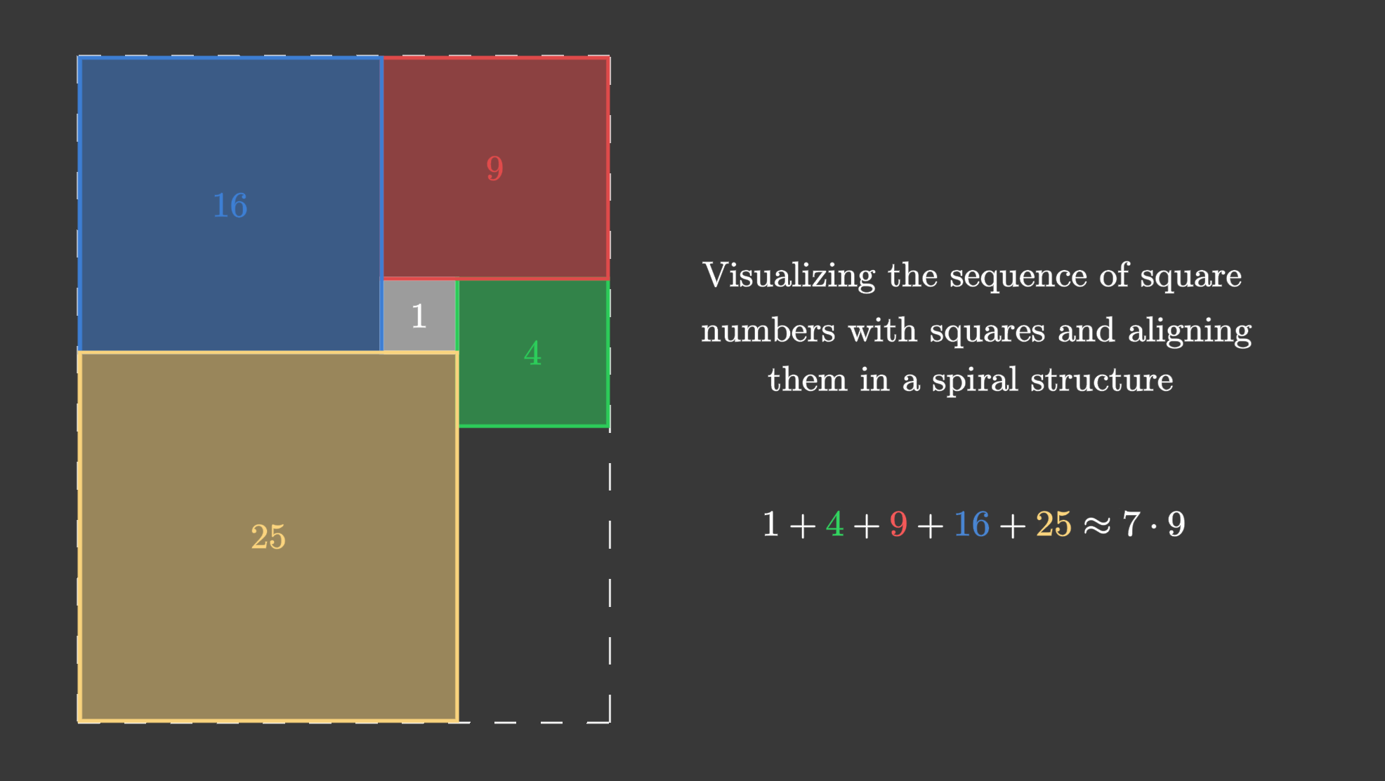
If we arrange these squares in a spiral-like pattern, we notice something intriguing: they almost fill a rectangle. One might therefore attempt to approximate the sum simply by computing the area of this rectangle. As the spiral is extended further, however, overlaps begin to appear —specifically, every four squares a new round of overlapping starts. Let us therefore continue the construction until the first overlaps occur.
Although these overlaps make the picture less tidy, the four preceding squares still combine to form a rectangle, as illustrated in the figure. This observation suggests a recursive structure, which is shown in more detail in the following diagram.
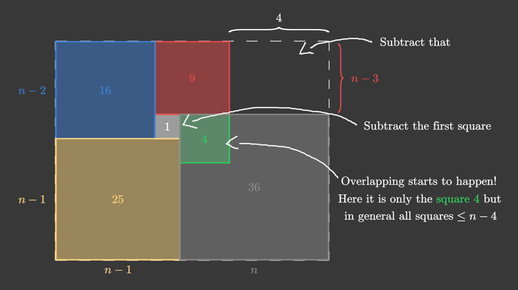
Suppose we want to compute the sum up to \(n = 6\). The area of the rectangle that nearly represents this sum has side lengths \(5 + 6 = 2n - 1\) and \(4 + 5 = 2n - 3\). This same relationship holds in general; you may verify this yourself by drawing the cases \(n = 7\) or \(n = 10\).
However, this rectangular area slightly overshoots the true sum. In the upper-right corner, we find a region that must be subtracted. The width of this smaller rectangle is always \(4\), while its height depends on \(n\) and is given by \(n - 3\).
Furthermore, the very first square of size 1, has to be subtracted too. It is contained in the rectangle but not part of the sum of the last 4 squares.
At this point, we have found a way to express the contribution of the last four square numbers. To obtain the full sum, we simply collect the remaining terms — those squares that already overlap — into the quantity \(S_{n-4}\). This leads us to the recursive relation — the area of the rectangle minus the upper right smaller rectangle minus 1 from the first square plus the remaining sum — as shown in the following equation
\begin{equation} S_n = (2n - 1)(2n - 3) - 4(n - 3) + S_{n-4} - 1. \end{equation}Expanding this expression yields a quadratic polynomial:
\begin{equation} S_n = 4n^2 - 12n + 14 + S_{n-4} \end{equation}Evaluating this recursion (with initial values \(0, 1, 5, 14\)) indeed reproduces the correct partial sums.
But what have we actually gained from this? Not very much — after all, we already had a recursive relation: moving from one partial sum to the next simply adds \(n^2\). Now we have merely expressed this recurrence in steps of four. While interesting, this does not yet give us a closed-form solution.
A function that satisfies the difference property
However, this recursive viewpoint does reveal something important: any closed-form sum must satisfy this recurrence. And in particular, also the one step recursion that is the difference of one step is just \(n^2\). In other words our function that yields the sum up to the \(n\)-th square number, must satisfy
\begin{equation} S_n - S_{n-1} = n^2 \end{equation}If we write the sum as a function \(f\) defined on the natural numbers, then our task reduces to finding a function such that
\begin{equation} f(n) - f(n-1) = n^2 \quad \forall n \in \mathbb{N} \end{equation}At first glance this may seem like nothing new. But in fact, such a function is not difficult to find. We do not have to find the function, we just have to find a function whereby at each \(n\)-th step yields \(n^2\). To begin, let us first revisit the simpler case studied by Gauss: the sum of the integers up to \(n\). There, we seek a function satisfying
\begin{equation} f(n) - f(n-1) = n \end{equation}A difference that produces a linear term suggests a quadratic function. Let us therefore try \(f(n) = n^2\) and compute
\begin{equation} n^2 - (n-1)^2 = 2n - 1 \end{equation}This is close, but not quite what we want. Scaling by a factor of \(\frac{1}{2}\) fixes the coefficient:
\begin{equation} \frac{n^2}{2} - \frac{(n-1)^2}{2} = n - \frac{1}{2} \end{equation}We are now only missing a constant term. This can be corrected by adding a linear term, since
\begin{equation} n - (n-1) = 1 \end{equation}Choosing \(f(n) = \frac{n^2}{2} + \frac{n}{2}\), we finally obtain
\begin{equation} \frac{n^2}{2} + \frac{n}{2} - \left[\frac{(n-1)^2}{2} + \frac{n-1}{2}\right] \end{equation} \begin{equation} n - \frac{1}{2} + \frac{n}{2} - \frac{n}{2} + \frac{1}{2} = n \end{equation}Thus, \(f(n)\) satisfies \(f(n) - f(n-1) = n\) and hence each value of \(f(n)\) will exactly yield the sum of the natural numbers up to \(n\), that is, \(\sum_{i=1}^n i\).
Expanding Gauss's original formula \((n+1)\frac{n}{2}\) confirms that both expressions are identical.
Of course, this is not the only function that satisfies the condition on the natural numbers. One could construct other functions that agree at integer points but oscillate wildly in between. For our purposes, however, a single such function is entirely sufficient — and this one we just found is likely the simplest one.
Let us now return to the sum of squares. We seek a function \(f\) such that
\begin{equation} f(n) - f(n-1) = n^2 \end{equation}Following the same strategy, we start with the next higher power, since the difference of a cubic will contain a quadratic term:
\begin{equation} n^3 - (n-1)^3 = 3n^2 - 3n + 1 \end{equation}Scaling again, we try \(f(n) = \frac{n^3}{3}\), which yields
\begin{equation} \frac{n^3}{3} - \frac{(n-1)^3}{3} = n^2 - n + \frac{1}{3} \end{equation}The unwanted linear term \(n\) can be eliminated by adding a quadratic term — coincidentally (or not?) exactly the expression corresponding to the sum of integers we have just found. Doing so gives
\begin{equation} f(n) = \frac{n^3}{3} + \frac{n^2}{2} + \frac{n}{2} \end{equation}This leaves us with a constant offset, which can be analogous to the previous derivation encountered with a linear term, in this case by \(-\frac{n}{3}\). This term can be collected together with \(\frac{n}{2}\), so we obtain
\begin{equation} f(n) = \frac{n^3}{3} + \frac{n^2}{2} + \frac{n}{6} \end{equation}A straightforward calculation confirms that
\begin{equation} f(n) - f(n-1) = n^2 \end{equation}and thus this function indeed represents the sum of the first \(n\) square numbers.
It is worth noting that this expression is usually written in a more compact, factorized form
\begin{equation} \frac{n(n+1)(2n+1)}{6} \end{equation}By expanding the above expression, one can quickly verify that it matches our derived polynomial.
Generalizing the Idea and Umbral Calculus
Naturally, this procedure can be extended further: sums of cubes, fourth powers, and higher powers can all be derived in the same way. To avoid the tedious algebra, one could even write a small program to carry out these steps automatically.
Even at this stage, certain patterns become visible. The sum of \(n^k\) is always a polynomial of degree \(k+1\). Alternative recursive relations — such as the one we found for steps of four in the square numbers — remain of the same degree but involve more complicated coefficients.
So what have we actually been doing here? Into which mathematical territory have we wandered?
This whole approach strongly resembles a form of discrete calculus. Indeed, equations of the form \(f(n) - f(n-1) = n^2\) are known as difference equations, the discrete analogues of differential equations. What we have effectively been doing is integrating discretely.
This is a lesser-known but deeply fascinating area of mathematics. Stirling wrote extensively on these ideas, most notably in Methodus Differentialis. A part of discrete calculus is also often referred to as umbral calculus — a name that fittingly reflects its somewhat mysterious character.
In this Story, we have already taken a small step into umbral calculus without explicitly naming it. The moment we began to search for a polynomial function whose finite difference reproduces a given sequence — rather than computing sums term by term — we adopted an umbral point of view. Instead of treating \(n^2\) merely as a sequence of numbers, we treated it as the shadow of a higher-degree polynomial under the finite difference operator. In the following image the two expressions we have just derived are visualized (interpreted as polynomial functions).
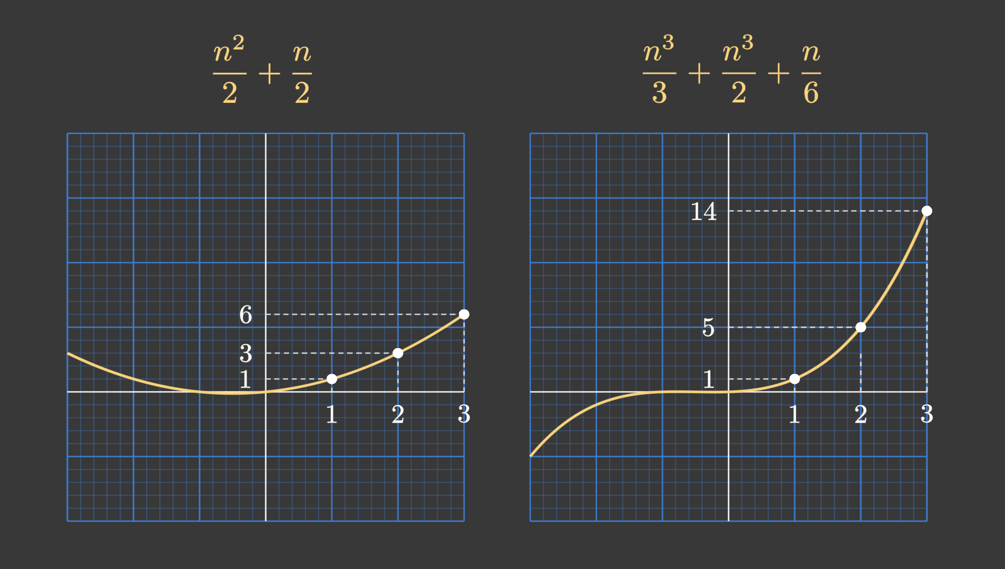
This shift in perspective is characteristic of umbral calculus: sequences are studied through the algebraic properties of the polynomials that generate them, and summation becomes the problem of finding discrete antiderivatives. What we have done here is therefore not the full machinery of umbral calculus, but a first glimpse of its core idea — that many summation formulas can be derived systematically by working with operators and polynomial structures rather than explicit sums.
Conclusion and Outlook
For this story, we will leave it here. But discrete calculus is a rich and powerful field, especially umbral calculus: it leads to approximation formulas for factorials, reveals special number sequences such as the Bernoulli numbers, and even connects to asymptotic (generally non-convergent) series like the Maclaurin series. It is an incredibly exciting area of mathematics — one we will certainly return to in future stories.