Introduction
What exactly is a vector? At first glance, this question may seem somewhat crude and simplistic. But in truth, it is anything but. A simplistic and superficial answer might be: some things can be represented by a single number, while others consist of multiple parameters, which can be expressed as a list of numbers. This list, when taken together, is often referred to as a vector. However, such an answer is far too brief and lacks depth. Why, for instance, can a vector be depicted as an arrow? And more intriguingly, why is it so often represented in this manner when a list of numbers would seemingly correspond to a mere point? Furthermore, how does one approach the addition of these entities that are presented as lists of numbers? Is it simply a matter of adding them element-wise, or is there something more profound at play?
It is exactly these kinds of curious questions that reveal why the simple explanation falls short. A vector is far more than a mere list of numbers. What makes something a vector is not what it looks like, but the logic it follows. This logic, a structured framework of rules known as a vector space, can encompass many kinds of elements; in some cases, even functions can form such a space. A vector is then simply an element of such a space. But let us start from the very beginning.
Graphical representation of a vector
Let us begin with the familiar image of an arrow and use this as a starting point to explore why this representation makes so much sense. For now, let us confine ourselves to the concrete example of a two-dimensional vector. With this simplification, the concepts become easier to grasp visually. Once we have established a solid understanding here, we can generalize to higher dimensions without significant difficulty. In the following illustration, a vector \((a,b)\) is depicted.
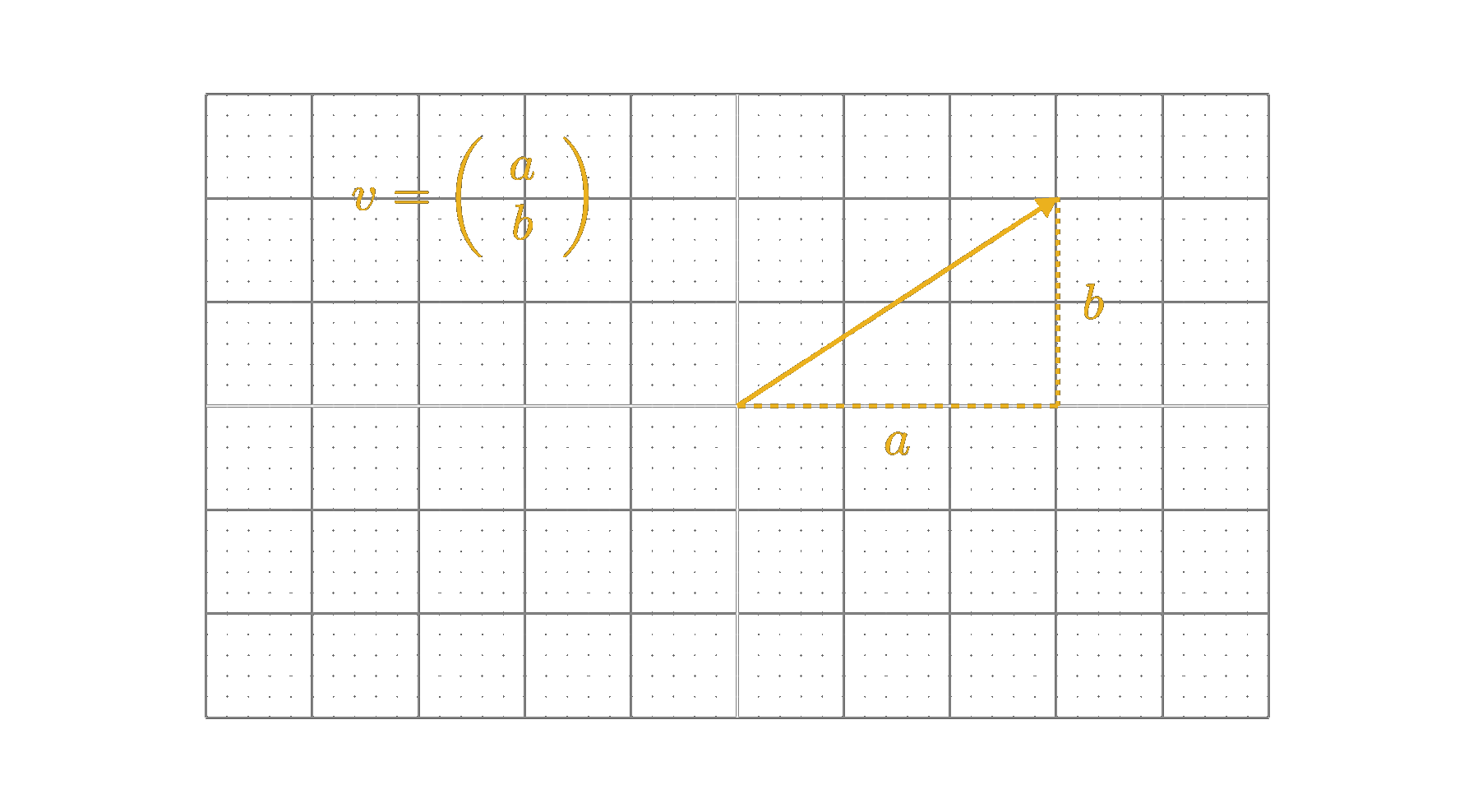
In the image above, we see that a vector is depicted as an arrow. This is because a vector inherently carries properties for which arrows are a good visual example. So when it comes to vectors, let us try not to think of a list of numbers, but rather of arrows that have a direction and a magnitude. One could sum this up by viewing vectors as a kind of displacement.
This perspective already answers one of our initial questions. A displacement is not tied to a particular location: moving three steps to the right and one step up is the same displacement, no matter where we start. Accordingly, all arrows with the same length and direction represent the very same vector, regardless of where in the plane they are drawn. A point, on the other hand, is a location. The two are related, but they are not the same: if we start at the origin and perform the displacement, we end up at a point, which is why the list \((a,b)\) can describe both. Conversely, the difference between two points is a displacement, namely the arrow leading from one to the other. A point says where something is; a vector says how to get somewhere.
With this change in perspective, we can now consider what happens if we add two displacements (perhaps by executing them one after the other). What happens if we subtract two displacements, or if we undo a displacement? Additionally, what exactly defines the direction of a displacement? Some displacements point in the same direction, while others do not. What are the consequences of this?
Operations on vectors
Let us begin with the first set of questions about operations like adding or undoing displacements. Here, the new perspective of displacements really pays off.
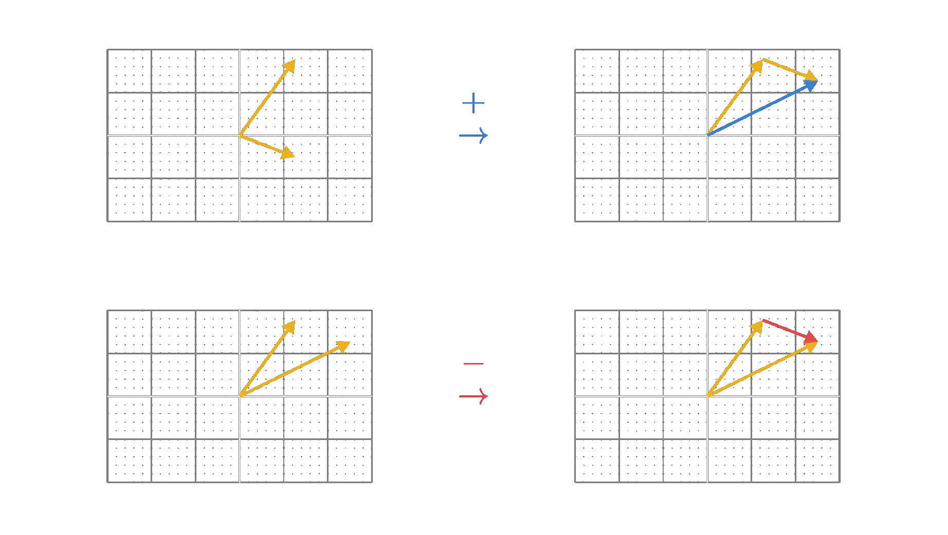
Starting with addition, we can simply interpret it as executing two displacements one after the other. The result can be easily determined by placing the tail of the second arrow at the tip of the first one. The tip of the second arrow then indicates where we end up after executing both displacements. The resulting displacement is the arrow from the tail of the first arrow to this end point.
Subtraction is the inverse of addition, so we are essentially asking: which displacement do I have to perform additionally to reach a given final displacement (that is, a given final arrow)? This turns out to be completely straightforward. Simply place the arrows of the first and the final displacement at the origin and draw a new arrow from the tip of the first arrow to the tip of the final arrow. This arrow is exactly the additional displacement we are looking for. The direction matters here: the reversed arrow would answer the opposite question. Both addition and subtraction are illustrated in the following figure.
Next, let us consider undoing a displacement. This corresponds to an arrow of the same length pointing in the exact opposite direction, which makes it a rather simple operation.
Now, what about scaling? Scaling a displacement by three simply means executing it three times. Visually, this corresponds to a new arrow composed of three copies of the original arrow. But the scaling factor does not have to be a whole number: scaling by \(\tfrac{1}{2}\) means going only half the way, and in general, scaling by any positive real number stretches or shrinks the arrow by that factor while keeping its direction. Scaling by a negative number additionally flips the arrow around. In particular, scaling by \(-1\) is exactly the same as undoing the displacement.
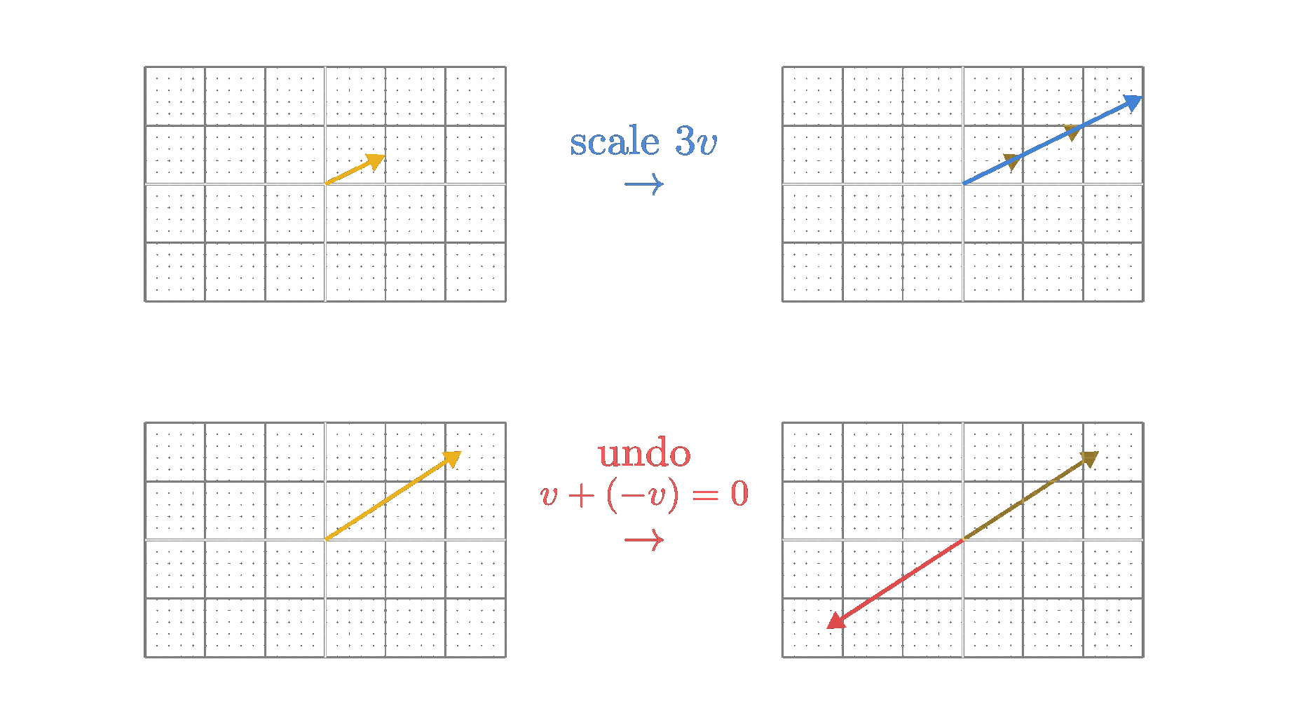
In the image above, both undoing and scaling are illustrated.
Logical structure
You might have noticed that for all the operations we have just derived, we did not need the idea of a list of numbers at all. We have only been talking about displacements. So, clearly, a vector cannot simply be a list of numbers. Perhaps it is not one at all? But then again, what exactly is a vector?
The key to understanding this is to view a vector (and perhaps nearly everything in mathematics) through the lens of a logical structure. The operations we have just defined? They are already what makes something a vector. To be rigorous, we need to add a few basic rules such as associativity, but that is essentially it. Any set whose elements can be added and scaled according to such a logical structure can be viewed as a set of vectors. This logical structure is known as a vector space, and its elements are called vectors.
For the sake of completeness, let us state precisely what is required. A vector space consists of a set \(\mathcal{V}\) together with two operations: an addition, which combines two elements of \(\mathcal{V}\) into a new element of \(\mathcal{V}\), and a scalar multiplication, which combines a scalar (for now, a real number) and an element of \(\mathcal{V}\) into a new element of \(\mathcal{V}\). For all \(u, v, w \in \mathcal{V}\) and all scalars \(a, b \in \mathbb{R}\), these operations must satisfy the following rules:
- associativity of vector addition: \(u + (v + w) = (u + v) + w\)
- commutativity of vector addition: \(u + v = v + u\)
- identity element of vector addition: there is a zero vector \(0 \in \mathcal{V}\) with \(v + 0 = v\) for all \(v \in \mathcal{V}\)
- inverse elements of vector addition: for every \(v \in \mathcal{V}\) there is a \(-v \in \mathcal{V}\) with \(v + (-v) = 0\)
- compatibility of scalar multiplication with field multiplication: \(a(bv) = (ab)v\)
- identity element of scalar multiplication: \(1v = v\)
- distributivity of scalar multiplication with respect to vector addition: \(a(u + v) = au + av\)
- distributivity of scalar multiplication with respect to field addition: \((a + b)v = av + bv\)
In our case, the set \(\mathcal{V}\) consists of all possible displacements in 2D. Naturally, this set contains infinitely many elements. The zero vector is the displacement that does not move at all, and \(-v\) is the undone displacement \(v\).
It is worth noting how easily these rules can be violated. Consider only those displacements that move at least a little to the right. Adding two of them again yields a displacement to the right, so far so good. But undoing such a displacement leads to the left, i.e. outside of our set. The inverse elements are missing (and so is the zero vector), so this set is not a vector space, even though its elements are exactly the same kind of arrows as before. Being a vector is therefore not a property of a single arrow, but of the whole set and of how its elements can be combined.
Furthermore, in a more general sense, the real numbers used as scalars can be replaced by something more general that again satisfies certain logical rules. This other logical structure is called a field and is usually denoted by \(K\). However, we will not dive into that generalization here.
Span, basis and linear independence
This vector space imposes some structure on the set \(\mathcal{V}\). Using the addition and the scalar multiplication, we can combine vectors into new ones. An expression like \(av + bw\), where \(a\) and \(b\) are scalars and \(v\) and \(w\) are vectors, is called a linear combination of \(v\) and \(w\). The set of all vectors that can be reached by linear combinations of some given vectors is called the span of these vectors. So navigating around in \(\mathcal{V}\) following the rules induced by the vector space naturally raises the question: which vectors can be reached from a given set of vectors, and which cannot?
Closely related is the question of whether some of the given vectors are redundant. If one of them can itself be written as a linear combination of the others, it adds nothing new to the span: everything it could contribute, the others can already reach on their own. If, on the other hand, none of the vectors can be written as a linear combination of the others, they are called linearly independent. Formally, vectors \(v_1, \dots, v_n\) are linearly independent if
\begin{equation} a_1 v_1 + a_2 v_2 + \dots + a_n v_n = 0 \end{equation}only holds when all scalars \(a_1, \dots, a_n\) are zero. Otherwise, they are called linearly dependent.
Let us put this into our visual setting of displacements. Imagine having two displacements that lie on the same line, so they point either in the same or in exactly opposite directions. One of them is just a scaled version of the other, so they are linearly dependent. If we combine them linearly (that is, scale and add them), we can reach any displacement along that line, but none that leaves it. So a huge chunk of the set \(\mathcal{V}\) remains inaccessible.
Now consider a different scenario: we start with two displacements that do not lie on a common line (and neither of them is the zero displacement). These two are linearly independent, and it turns out that we can reach any possible displacement by linearly combining just these two. Suddenly, their span is the entire set \(\mathcal{V}\).
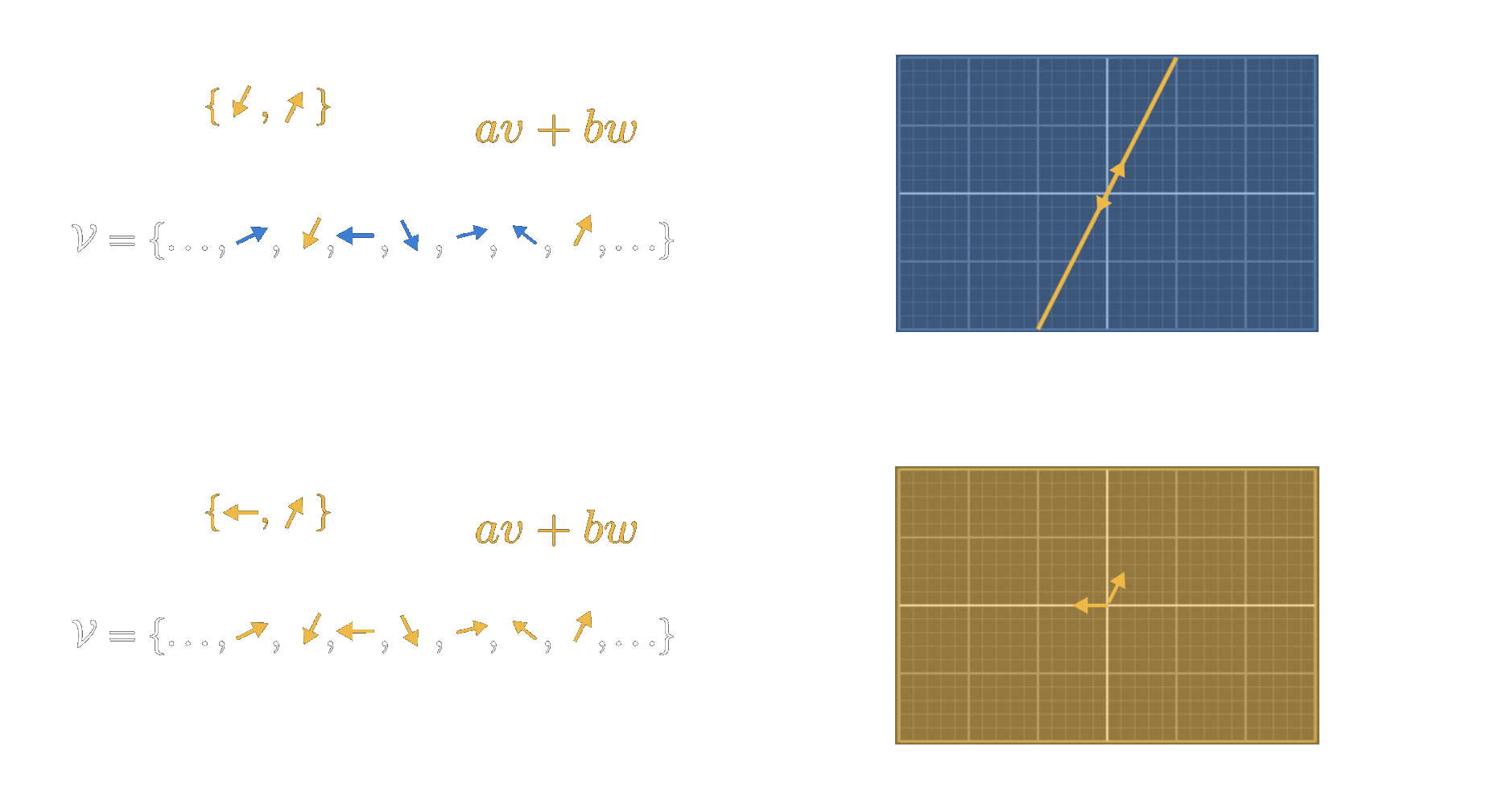
A set of vectors that is linearly independent and whose span is the entire set \(\mathcal{V}\) is called a basis of the vector space. Equivalently, a basis is a spanning set that is as small as possible: if we removed any one of its vectors, part of \(\mathcal{V}\) would become unreachable. Needless to say, there are usually endless possibilities to choose a basis for a vector space.
Let us return to the image from the very beginning and interpret basis and span in this concrete visual context, so \(\mathcal{V}\) will be \(\mathbb{R}^2\). The two vectors that point along the axes, each corresponding to one unit in its respective direction, are the basis vectors. Together they form the so-called standard basis. The coordinate grid brilliantly shows their possible linear combinations (restricted to integer scalars, or at least to some finite level of granularity).
Now, what happens if we change this basis? As mentioned above, there are usually infinitely many bases for a vector space. In our example, we can choose any two vectors that do not lie on a common line. Let us pick two random ones. What would we need to do to transform every element from its representation in the original basis to the new one? We can simply express the original basis vectors as linear combinations of the new basis vectors. Then we can take any vector written as a linear combination of the original basis vectors and replace those with their corresponding linear combinations of the new basis vectors. This process is called change of basis, and the following image illustrates it using our example of \(\mathcal{V}=\mathbb{R}^2\).
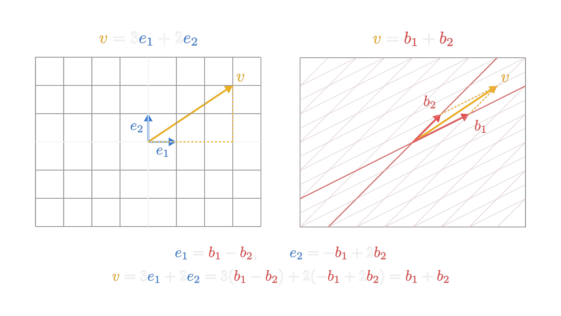
Finally, we can return to our list of numbers and see what it is all about. The numbers are just the scalars by which we have to scale the basis vectors in the linear combination to reach a particular vector. Linear independence guarantees that these scalars are unique: if a vector could be written in two different ways, subtracting the two linear combinations would give a linear combination of the basis vectors that equals zero without all scalars being zero, which is impossible for linearly independent vectors. So once a basis is fixed, every vector corresponds to exactly one list of numbers, and every list of numbers to exactly one vector. The order matters as well: the first number belongs to the first basis vector, the second number to the second, and so on.
Needless to say, a vector is not this list of numbers. The list is merely a shorthand notation, namely the vector's coordinates with respect to a basis. In particular, without explicitly stating which basis the numbers refer to, they are completely useless. Usually, of course, it is implied that they refer to the standard basis, represented by the standard coordinate grid we are all familiar with.
This also answers another question from the introduction: why are vectors added element-wise? Let \(e_1\) and \(e_2\) be our basis vectors, and let \(u = x_1 e_1 + y_1 e_2\) and \(v = x_2 e_1 + y_2 e_2\). Using only the rules of the vector space (in particular associativity, commutativity and the two distributive laws), we obtain
\begin{equation} u + v = (x_1 + x_2)\,e_1 + (y_1 + y_2)\,e_2 \end{equation}and, for any scalar \(c\),
\begin{equation} c\,u = (c\,x_1)\,e_1 + (c\,y_1)\,e_2. \end{equation}So adding coordinates element-wise and multiplying each coordinate by the scalar is not an arbitrary definition; it is a direct consequence of the vector space rules. And it works in any basis, not only in the standard one.
Generalizing to higher dimensions
Up to this point, we have focused mostly on two-dimensional vectors, since they are easy to visualize as arrows in the plane. But notice something important: when we defined the logical structure of a vector space, we never once mentioned "dimension". Yes, for the visualization we used two-dimensional arrows. However, none of the rules of addition and scalar multiplication required us to be in two dimensions. We used the notion of displacements to get a feeling for those rules, but we could just as well have used any other abstract thing that follows them.
So what exactly is a dimension in the context of a vector space? On the most foundational, abstract level, the dimension of a vector space is simply the number of elements in a basis. In other words, it is the maximum number of linearly independent vectors the space can contain. That this is well-defined is not obvious at all: a vector space has many different bases, so why should they all have the same size? It is a fundamental theorem of linear algebra that they do. Every basis of a given vector space contains the same number of vectors, and only because of this does it make sense to speak of the dimension of a space.
For a two-dimensional vector space, two basis vectors are enough to reach every possible displacement. In a three-dimensional one, we need three. In general, if a space requires \(n\) independent directions to span it, we call it an \(n\)-dimensional space.
From this point of view, moving to higher dimensions is straightforward: all of the logic we developed in two dimensions (addition, scaling, span, basis, linear independence) carries over directly, because, as we saw, we did not even need the concept of a dimension to define them. The only obstacle might be our imagination. While we can picture vector spaces of three or fewer dimensions with arrows, it is impossible to do the same for four or even ten dimensions. Mathematically, however, nothing changes. As long as the logical rules are followed, we can treat the set as a vector space, or, more precisely, it then is a vector space, no matter whether two, four or ten elements are required to span the whole set \(\mathcal{V}\). There are even vector spaces in which no finite number of vectors suffices, for example the space of all polynomials. These are called infinite-dimensional, and we will catch a glimpse of one in the next section. Dimension is simply a measure of how much independence there is in the space, not a limit to the vector concept itself.
Abstract vector spaces
So far, our concrete examples of vectors have been displacements in space. But the power of the vector space concept is that it applies to far more abstract situations as well. It is a logical structure that can arise all over the place, and any kind of object can be viewed as a vector, as long as it is part of a set that follows the rules of a vector space.
A particularly striking example comes from the world of oscillations. Consider the two functions
\begin{equation} f_1(t) = \sin(t), \qquad f_2(t) = \cos(t). \end{equation}At first glance, these look nothing like arrows or displacements. Yet, from the right perspective, they behave in just the same way: they form a basis of a vector space of oscillations. How? If we take any linear combination
\begin{equation} a\,\sin(t) + b\,\cos(t), \end{equation}where \(a, b \in \mathbb{R}\), we again obtain a function. Adding two such functions or scaling one of them yields a function of exactly the same form, and all the rules of a vector space follow directly from the familiar rules for adding and multiplying real numbers. The zero vector is the function that is zero everywhere, which we can think of as an oscillation with amplitude zero. Checking the individual rules in detail is a nice exercise, which we will leave to you.
But do all of these functions really represent oscillations, and can every oscillation be written in this form? Not every oscillation: all of these functions oscillate with the same frequency as \(\sin(t)\) and \(\cos(t)\) themselves. An oscillation with a different frequency, such as \(\sin(2t)\), cannot be written in this form. Within this fixed frequency, however, the answer is yes in both directions. Using the angle addition identity,
\begin{equation} R\,\sin(t + \phi) = R\cos(\phi)\,\sin(t) + R\sin(\phi)\,\cos(t), \end{equation}we see that an oscillation with amplitude \(R\) and phase shift \(\phi\) is a linear combination of \(\sin(t)\) and \(\cos(t)\) with \(a = R\cos(\phi)\) and \(b = R\sin(\phi)\). Conversely, for any \(a\) and \(b\) that are not both zero, we can choose \(R = \sqrt{a^2 + b^2}\) and \(\phi\) such that \(\cos(\phi) = a/R\) and \(\sin(\phi) = b/R\). Then \(a\,\sin(t) + b\,\cos(t) = R\,\sin(t + \phi)\) is a pure oscillation with amplitude \(R\) and phase shift \(\phi\).
Look closely at these formulas, because they hide a beautiful connection to the arrows from the beginning. If we draw the coordinates \((a, b)\) of an oscillation as an arrow in the familiar plane, this arrow has length \(R\) and points at angle \(\phi\). The amplitude of the oscillation is the length of the arrow, and its phase is the arrow's direction. Changing the amplitude corresponds to scaling the arrow, and shifting the phase by an additional angle corresponds to rotating the arrow by that angle. In this sense, our oscillations really are arrows in disguise.
It remains to check that \(\sin(t)\) and \(\cos(t)\) are linearly independent, i.e. that neither of them is just a scaled version of the other. Suppose \(a\,\sin(t) + b\,\cos(t) = 0\) holds for all \(t\). Inserting \(t = 0\) yields \(b = 0\), and inserting \(t = \pi/2\) yields \(a = 0\). So the only linear combination that gives the zero function is the trivial one, and the two functions indeed form a basis. Incidentally, the same trick shows why \(\sin(2t)\) is not in their span: if \(\sin(2t) = a\,\sin(t) + b\,\cos(t)\) held for all \(t\), inserting \(t = 0\) and \(t = \pi/2\) would again force \(a = b = 0\), yet \(\sin(2t)\) is clearly not the zero function.
Here, too, it is instructive to see how easily the vector space structure can break. Consider only the oscillations with an amplitude of exactly \(1\). Adding \(\sin(t)\) and \(\cos(t)\) yields \(\sqrt{2}\,\sin(t + \pi/4)\), an oscillation with amplitude \(\sqrt{2}\), which lies outside of this set. The zero function is missing as well. So the oscillations with a fixed amplitude do not form a vector space, while all oscillations of a fixed frequency do.
And if we allow all frequencies at once, that is, all linear combinations of \(\sin(nt)\) and \(\cos(nt)\) for \(n = 1, 2, 3, \dots\), we no longer get by with finitely many basis vectors. This is exactly the kind of infinite-dimensional vector space mentioned before, and it is the starting point of Fourier analysis.
Summary and outlook
That was quite a journey! We touched on one of the most foundational concepts in mathematics, moving beyond the classical picture of arrows to an abstract, logical structure. More precisely, mathematicians refer to this as an algebraic structure. However, throughout this story, we chose to use the term logical structure, as it better captures the underlying idea and helps build an intuitive understanding.
Now, there is one last question you might still be wondering about: what about multiplication? The dot product? Is that not also part of a vector space? Actually, no. According to the formal definitions used in mathematics, the logical structure we discussed above (addition, scaling, linear combinations) is already all it takes to be a vector space. At its core, this is what vectors are truly defined by. Nothing more is needed.
However, the familiar Euclidean plane, with vectors represented as arrows, is actually more than just a vector space. It belongs to a richer structure known as an inner product space, where concepts like length, angle and the dot product become meaningful. In fact, you have already caught a glimpse of it: the amplitude \(\sqrt{a^2 + b^2}\) of our oscillations is exactly such a length.
But that... is a story for another time. For now, we will leave it here.