Introduction
The normal distribution is arguably the most important probability distribution of all. It acts as a kind of fixed point toward which any sum of random variables tends to converge. In other words, no matter what distribution you start with (as long as its variance is finite to be precise), if you look at the sum of many independent samples from that distribution, the resulting distribution will approach a normal distribution. But why should such a “fixed point” distribution exist in the first place? And what about its shape? Why does its formula involve both \(\pi\) and \(e\)? Where does the circle come in, and what does it have to do with exponentials?
In this Story, we will explore these questions by retracing the original discovery of the normal distribution. In particular, we will follow the path Gauss took to arrive at this remarkable equation
\begin{equation} f(x) = \frac{1}{\sigma \sqrt{2\pi}} \, e^{ -\frac{(x - \mu)^2}{2\sigma^2} }. \end{equation}By modern standards, Gauss's derivation may lack full mathematical rigor. Nevertheless, retracing the reasoning of someone who had no prior knowledge of the normal distribution (at least not in the sense of its importance) is an enlightening experience. Approaching it in this spirit of discovery can lead to a much deeper understanding of what the normal distribution really is. Of course, this is only one perspective — Gauss's perspective. But combining this historical approach with a solid understanding of the central limit theorem and probability theory as a whole can provide a much richer and more intuitive grasp of the normal distribution. So, without further ado, let us dive in.
Historical background
The year is 1809, and Gauss publishes his monumental work Theoria motus corporum coelestium in sectionibus conicis solem ambientium (“Theory of the Motion of the Heavenly Bodies Moving about the Sun in Conic Sections”). In it, he dedicates a chapter to estimating the orbital parameters of celestial bodies. These estimates are based on real astronomical observations.
Such astronomical observations are always only so accurate. So, needless to say, they cannot be taken as the absolute truth down to the last decimal. They are inevitably affected by errors. These errors are random and arise from many sources: atmospheric effects such as heat shimmer, imperfections in the instruments, and even the limitations of human observers, who can only point the telescope's reticle with a certain degree of precision.
The central problem Gauss faced was this: how do we determine the orbital parameters from observations that are all corrupted by error? In fact, this determination is less a simple “calculation” but actually an “estimation” — and that is how also Gauss referred to it. So let us examine this in more detail.
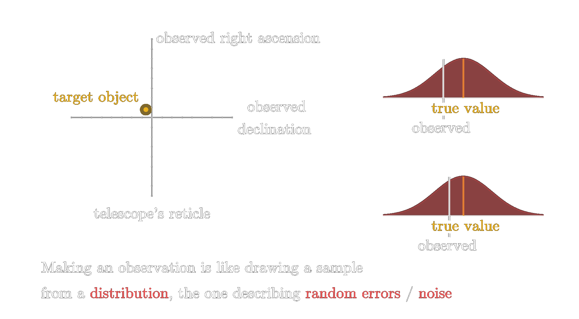
As shown in the image above, each observation is not a single exact value, but rather one sample from an unknown distribution of possible errors — a distribution that describes all the random influences that cause the observation to deviate slightly from the true value (a value known only to an omniscient observer). Each time we make an observation, we are essentially taking one random draw from this error distribution. Sometimes we are lucky, and the value is very close to the truth. Sometimes we are less lucky, and the value is farther away. But, how can we then find the correct solution to the orbital parameters if everything is based on chances?
Obviously, the first thing we can easily agree on: the more observations we collect, the better. A single measurement tells us very little about the true value — it might be perfectly accurate by coincidence, or it might be an outlier. If we gather, say, twenty independent observations, we reduce the risk of being misled by a single extreme error. But the question remains: given these twenty measurements, how should we combine them to obtain the best possible estimate of the orbital parameters? In other words, how do we “fit” an orbit to the data points in a principled way?
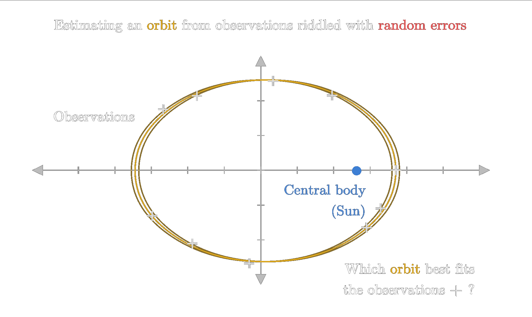
To have any chance of finding the best estimate, we would first need to know what distribution these random errors follow. Without that information, we are just left fumbling in the dark. But how could we possibly determine that distribution? The errors result from a combination of atmospheric turbulence, imperfect instruments, and human limitations — and that is all we know — a very vague and completely insufficient description. How could we find out about the shape of this error distribution, let alone deduce an exact equation for it?
And yet, Gauss did exactly that. From this vague picture and a few additional handful of basic, common-sense assumptions, he managed to derive an explicit formula for the distribution of errors — the formula we now know as the probability density function of the normal distribution. Incredible as it sounds, this is exactly what he achieved. So, let us see how he did it.
At the beginning Gauss lays out the problem in detail. Let us have a look at the original writing
The Setup
Gauss first discusses how to determine an orbit from exactly four observations. He then elaborates on what to do when there are more observations than strictly necessary to determine the orbital parameters. In particular, he writes:
Let \(V, V', V''\), etc. be functions of the unknown quantities \(p, q, r, s,\) etc., and let \(\mu\) be the number of such functions and \(v\) the number of unknown quantities. Suppose that the values of these functions obtained from direct observation are \(V = M, V' = M', V'' = M''\), etc. In general, determining the unknown quantities constitutes a problem that may be indeterminate, determinate, or overdetermined according as \(\mu < v, \mu = v,\) or \(\mu > v.\) We shall confine ourselves here to the last case, in which an exact representation of all the observations would be possible only if they were entirely free from error.
Let us put this into the context of orbit determination. By Gauss's time, it was well established — thanks to Kepler — that celestial bodies follow elliptical orbits. Thus, the general shape of the orbit was known. What remained was to determine the specific ellipse for a given body.
An ellipse in space is fully described by six parameters: the semi-major axis \(a\) and eccentricity \(e\) (or alternatively, \(a\) and \(b\) for the two axes), three angles that define the orientation of the orbital plane in three-dimensional space (inclination \(i\), longitude of the ascending node \(\Omega\), and argument of perihelion \(\omega\)), and finally, the position of the body on that orbit at a given reference time — often expressed as the time of perihelion passage \(T\) or as an additional angle called true anomaly \(v\) pointing to the current position in the elliptical orbit.
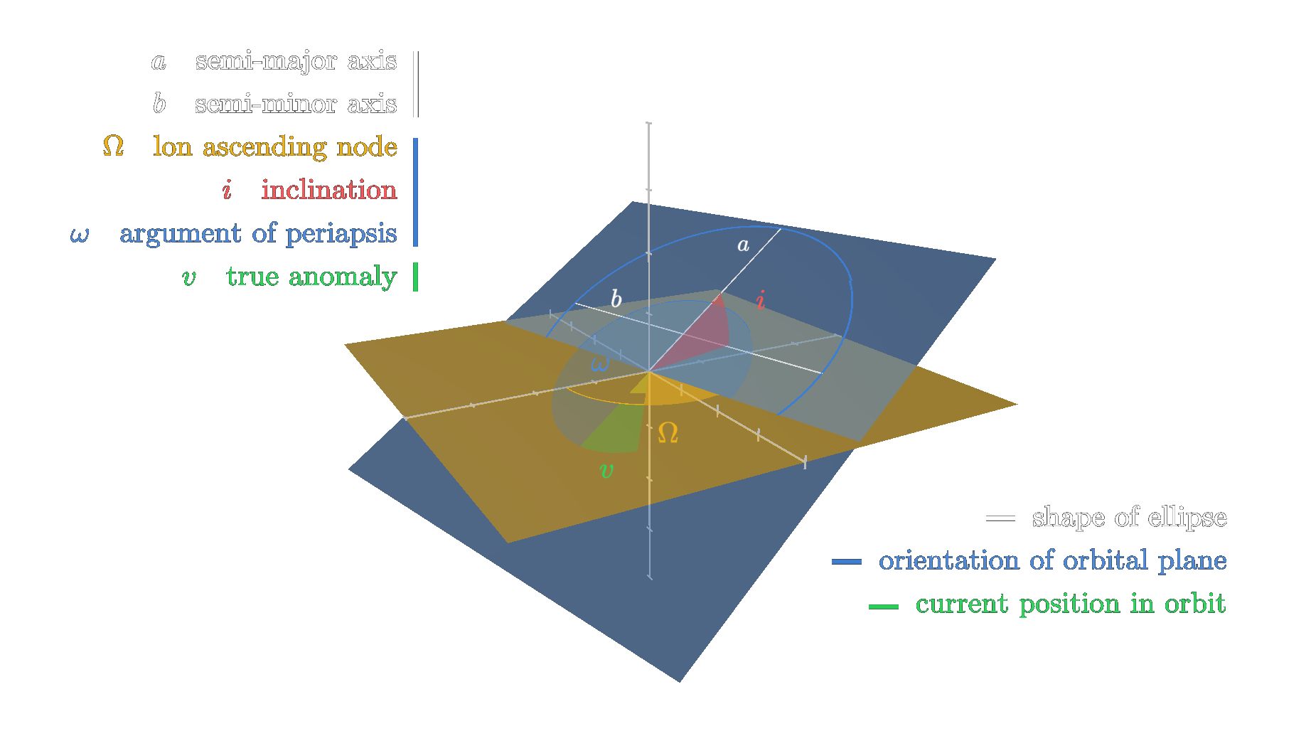
In Gauss's notation, the parameters \(p, q, r, s,\) etc. correspond to these six orbital parameters. The functions \(V\) of these parameters represent the predicted observations — usually the apparent position of the body on the celestial sphere, which astronomers measure as two angles: right ascension and declination (or equivalently, ecliptic longitude and latitude). For each observation, there are therefore two such functions, one for each angle.
With six parameters to determine, three observations (each yielding two equations) would give exactly enough information — the case \(\mu = v\) (here \(v\) referes to Gauss's text NOT the true anomaly). But as Gauss points out, we are interested in the case where there are more observations than unknowns (\(\mu > v\)), leading to an overdetermined system. This is exactly the situation astronomers face in practice: they collect as many observations as possible to reduce the effect of outliers while knowing that they cannot all be satisfied exactly because of observational errors.
Gauss now considers the situation where there is no reason to distrust any observation more than another. In other words, each measurement is assumed to be of equal precision, and errors of equal magnitude are equally likely in either direction. He writes:
Let us suppose, in the first place, that there is no reason to suspect one observation of being less exact than another, and that errors of equal magnitude are equally probable in all. The probability to be assigned to each error \(\delta\) will therefore be expressed by some function of \(\Delta\), which we shall denote by \(\varphi(\Delta)\).
Gauss denotes the probability density function of these random errors by \(\varphi(\Delta)\). Here, however, we will use the modern notation \(f(x)\) for this function. Keep this in mind if you plan to read Gauss's original text alongside this one. With that clarified, let us now see how Gauss derived an explicit form for this intriguing function describing random errors.
Gauss's Assumptions About Random Errors
The exact distribution of observational errors might at first seem impossible to guess. Nevertheless, Gauss made several reasonable and remarkably powerful assumptions about their nature:
- Existence of a true value: There is some true quantity around which all errors are distributed.
- Symmetry: Positive and negative errors of the same magnitude are equally likely, so the probability function is symmetric: \(f(x) = f(-x)\).
- Optimal estimation by the mean: Given multiple observations, the best estimate of the true value is the sample mean of the observations.
- Smaller errors are more likely than larger ones: The probability function must be monotonically decreasing as \(|x|\) increases (except at the center, where it reaches its maximum).
- Regularity: The function is smooth and differentiable (at least almost everywhere).
At first glance, many different functions seem to satisfy these five requirements. For example, a triangular distribution, a Laplace (double exponential) distribution, or even some odd strictly falling wave pattern distribution would seemingly meet all of them. In the following image such distributions are illustrated.
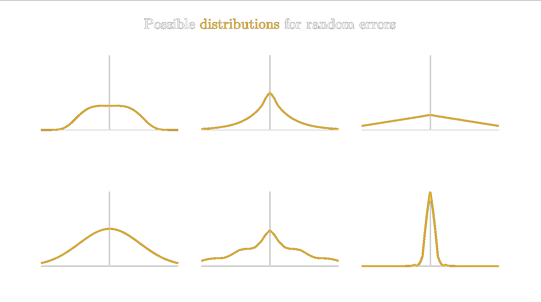
However, actually it turns out that the third assumption — that the sample mean is the most probable estimate — is extraordinarily strong. When combined with the other assumptions, it already uniquely determines the functional form of \(f(x)\). In other words, these conditions single out one particular function: the one we now call the normal distribution. This hints at the strong bond between the normal distribution and least squares, because the sample mean is the best estimate regarding least squares. If you wonder what least squares is, we will come back to it later in the Story.
But how did Gauss now actually derive his distribution and showed that those assumptions are already enough to pin it down to one particularly shaped curve only?
Gauss's Derivation
Let us denote the probability distribution function of the unknown error curve as \(f(x)\). From the second assumptions we get
\begin{equation} f(x) = f(-x). \end{equation}Gauss goes then on and considers the liklihood of a set of measurements. So imagine we have \(n\) observations, so \(n\) drawn samples, which we shall denote as \(X=(x_1, \dots, x_n)\). If we assume for one second that we knew the true value \(T\) we could compute the probability for that event, which we shall denote as \(\Omega\).
\begin{equation} \Omega = f(x_1-T)\cdot f(x_2-T)\cdot\quad\dots\quad\cdot f(x_n-T). \end{equation}Gauss interpreted the third assumption in a way that estimating \(T\) with the mean \(\bar{x}\), maximizes \(\Omega\). This means \(P(X)\) has a maxima at \(\bar{x}\). In other words the derivative with respect to \(T\) at this point is zero, which we can compute using the product rule
\begin{equation} \begin{aligned} \frac{\partial\Omega}{\partial T}|_{\bar{x}} = f'(x_1-\bar{x})f(x_2-\bar{x})\cdot\dots\cdot f(x_n-\bar{x}) \\ - f(x_1-\bar{x})f'(x_2-\bar{x}) \cdot\dots\cdot f(x_n-\bar{x}) - \quad\dots\quad \\ - f(x_1-\bar{x})f(x_2-\bar{x})\cdot\dots\cdot f'(x_n-\bar{x}) = 0 \end{aligned} \end{equation}At first glance, this step may feel very like waving the hand. Why can we just replace \(T\) with \(\bar{x}\) and why should the sample mean be the point of maximum? After all, \(\bar{x}\) will not, in general, be equal to \(T.\) It is only in the limit — when the number of samples goes to infinity — that \(\bar{x}\) converges to \(T\). In that idealized case, the \(x_i\) perfectly reflect the distribution of random errors, with no outliers remaining because the sample is infinite. And okay, even with a large but finite sample, the error that is made by assuming \(\bar{x}=T\) becomes miniscule small but a strict equality would still not be fully correct.
However, this limiting argument is *not* what Gauss is relying on. He is not assuming that the sample mean \(\bar{x}\) equals the true value \(T\). Instead, when he notes that the likelihood is maximized at \(\bar{x}\) — where its derivative is zero — he is making a different point: given the observed samples \(x_i\), if we shift the underlying probability distribution so that its mean is located at the sample mean, then the probability of observing *this particular* set of measurements is maximized.
In other words, Gauss interprets assumption 3 — that the sample mean is the best estimate of \(T\) — through the lens of maximum likelihood. The sample mean \(\bar{x}\) will typically not match \(T\) exactly, but it identifies the value of the distribution's mean that makes the observed data as likely as possible.
Of course, this maximum-likelihood interpretation does not come with a rigorous proof at this stage; it is essentially an informed guess by Gauss. Nevertheless, it is far from unreasonable. As we will see later, this viewpoint is closely connected to the method of least squares: the sample mean is indeed the optimal estimator in the least-squares sense. In this way, Gauss's argument proceeds in a kind of reverse direction: he first assumes that the sample mean serves as the maximum-likelihood estimator, then derives the corresponding error distribution and finally shows that for this distribution the maximum-likelihood estimate is indeed obtained by the method of least squares — thus lending support to the original assumption. This is, of course, a circular line of reasoning, but it at least shows that once the assumption is made, all subsequent results fit nicely together.
Accepting the lack of rigor and continuing with the derivation, assumption 5 ensures that the derivative of \(f\) — which we have just set to zero at the sample mean — indeed exists. Moreover, if you look at the previous equation, you will notice that we can factor out \(\Omega\), which leads to
\begin{equation} \Omega \left[ - \frac{f'(x_1-\bar{x})}{f(x_1-\bar{x})} - \frac{f'(x_2-\bar{x})}{f(x_2-\bar{x})} - \quad\dots\quad - \frac{f'(x_n-\bar{x})}{f(x_n-\bar{x})} \right] = 0 \end{equation}Obviously, the frequency of \(\Omega\) cannot be 0, otherwise the actual outcome would not have happened. Therefore we conclude
\begin{equation} \frac{f'(x_1-\bar{x})}{f(x_1-\bar{x})} + \frac{f'(x_2-\bar{x})}{f(x_2-\bar{x})} + \quad\dots\quad + \frac{f'(x_n-\bar{x})}{f(x_n-\bar{x})} = 0 \end{equation}Independent of what actual sample we had drawn we could made above conclusions. This means above equation being equal to 0 must hold for all abritrary sets of \((x_1, x_2, \dots, x_n)\).
We have now already found an interesting equation that must hold for our probability density function \(f.\) But is that already enough such that we can find an exact formula for it? Let us start by thinking more deeply about how the function \(f\) could look like such that above stated condition is actually fullfilled.
The most obvious canditate for \(f\) is needless to say where the derivative \(f'\) is zero everywhere. Then above sum will always evaluate to zero for all possible \((x_1,x_2,\dots,x_n)\). However this would leave only a constant function
\begin{equation} f(x) = const. \end{equation}as an equation for the probability density function. Obviously, this clashes with assumption 4, and would anyway make very little sense.
But are there any other possible solutions for \(f\) beside this trivial one. Let us examine above sum further. What we actually have here is that the values of a function evaluated at certain points have to sum to zero. This function is \(\frac{f'(x)}{f(x)}\). Let us denote it with \(\Phi(x)\), so we get
\begin{equation} \Phi(x_1-\bar{x}) + \Phi(x_2-\bar{x}) + \dots + \Phi(x_n-\bar{x}) = 0. \end{equation}It should now be clear that the set of functions \(\Phi\) that satisfy this requirement for all possible sets \((x_1, x_2, \dots, x_n)\) is actually quite limited. Let us visualize this idea to see why that is the case.
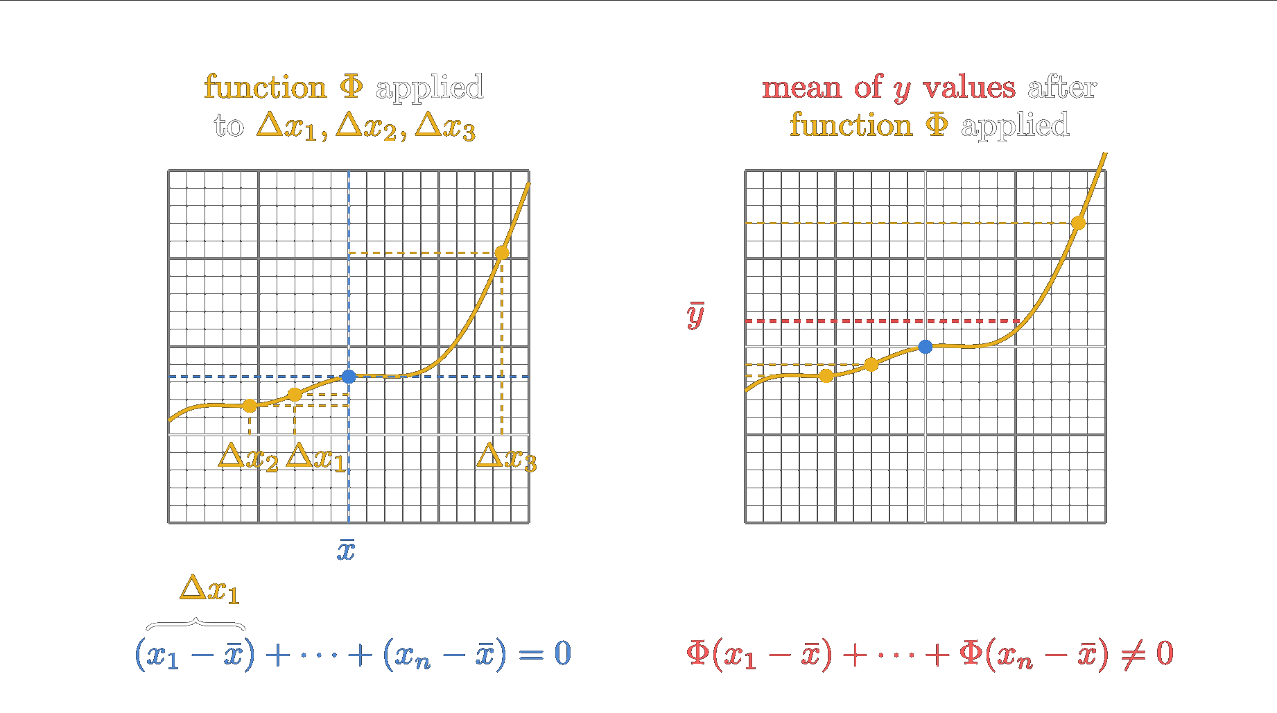
Suppose we have drawn three samples, \(x_1, x_2,\) and \(x_3\). We compute their mean, \(\bar{x}\), and determine the deviations of each sample from that mean, which we will denote as \(\Delta x_1, \Delta x_2,\) and \(\Delta x_3\). By definition, these deviations must sum to zero — otherwise, \(\bar{x}\) would not be the mean.
Now, if we look at the condition imposed on our function \(\Phi\), we notice that it involves the sum of all deviations after being transformed by \(\Phi: x \rightarrow \Phi(x)\). In essence, the requirement says that for any sample you take, the deviations from its sample mean — which already sum to zero — must still sum to zero after being mapped through \(\Phi\).
As you can see in the figure above, this is almost never the case for an arbitrary function. The example shown consists of a sinusoidal part combined with an overall upward curvature. When we map the deviations through this function to the \(y\)-axis, we can see that all resulting \(y\)-values lie on the positive side — so their sum clearly cannot be zero. Even if we shift the function so that it passes through zero at the mean (as illustrated on the right-hand side of the figure), the deviations \(\Delta x_1\) and \(\Delta x_2\) are compressed toward the mean, while the third deviation remains roughly the same distance from it. As a result, the transformed deviations no longer balance each other, and their sum becomes slightly positive.
Remember, this condition — that the transformed deviations (the \(y\)-values) must also sum to zero — must hold for any possible set of samples \((x_1, \dots, x_n)\). By now, maybe you can see what kind of functions this constraint allows. First, the function must pass through the origin; otherwise, there is always the possiblity that all \(y\)-values would lie entirely on one side of the axis, making their sum nonzero. Second, the function cannot have any curvature, since curvature would distort the spacing of the deviations unevenly, breaking the balance and shifting the mean away from zero.
Therefore, the only class of functions that meets this condition is:
\begin{equation} \Phi(x)=kx. \end{equation}Such a function always preserves the mean of the deviations because it represents nothing more than a scaling transformation — a change of units. For example, if a set of distances measured in meters sums to zero, those same distances measured in millimeters will also sum to zero. Or, to put it more vividly, if a balance scale is in perfect equilibrium with weights labeled in kilograms, it will, needless to say, remain balanced even if we relabel those weights in grams. The relationship is purely linear — and that is exactly what the condition demands.
Now that we have established this result, what does it imply for our function \(f\)? Recall that \(f\) is the probability function describing random errors we want to find an equation for. Let us express what the condition for \(\Phi\) tells us about \(f\):
\begin{equation} \Phi(x) = \frac{f'(x)}{f(x)} = kx. \end{equation}This gives us a differential equation for \(f\). It is actually a very simple one, and we can solve it directly. Let us begin by integrating both sides with respect to \(x\):
\begin{equation} \int\frac{f'(x)}{f(x)}dx = \int kx,dx. \end{equation}By substituting \(u = f(x)\), we note that \(f'(x)dx = du\). Performing the straightforward integration on the right-hand side, we obtain:
\begin{equation} \int\frac{1}{u}du = k\frac{x^2}{2} + C_1. \end{equation}The integral of \(1/u\) is the natural logarithm, so we have:
\begin{equation} \ln(u) + C_2 = k\frac{x^2}{2} + C_1, \end{equation}which, after exponentiating and recalling that \(f = u\), gives:
\begin{equation} f = e^{k\frac{x^2}{2} + C_3}. \end{equation}Since the exponential of a constant is just another constant, we can simplify this expression to:
\begin{equation} f = C e^{k\frac{x^2}{2}}. \end{equation}At this point, we have found the general functional form of \(f\). This is really an unbelievable and astonishing result. Just by making some vague trival assumptions about those random errors we were able to find this specific equation.
However, before celebrating to much, let us have a closer look at those set of functions that follow this equation by visualizing them. In the following image a few examples of how those functions look like are shown using different values for \(k\) and \(C\).
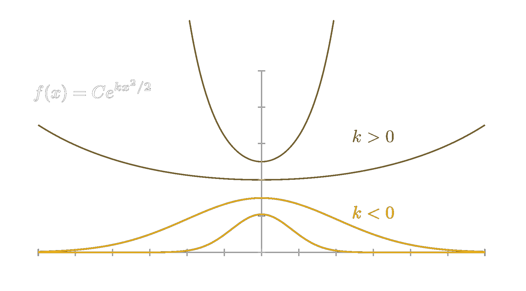
As can be seen in above figure, the constant \(C\) does not really do much other than scaling the graph and it essentially just determines where the function intersects the \(y\)-axis.
However, the impact of \(k\) is quite dractic. The shape of the error curve depends strongly on whether \(k\) is positive or negative. When \(k\) is positive, the function grows exponentially as we move away from the \(y\)-axis, meaning large errors become more and more probable. This clearly contradicts assumption 4 — that smaller errors should be more likely than larger ones. Therefore, we must restrict \(k\) to negative values only. Gauss expresses this by defining \(k/2=-hh\), whereby he writes about \(h\) the following:
Finally, the constant \(h\) can be considered as the measure of precision of the observations.
And indeed, it more or less corresponds to the today used notion of the standard deviation \(\sigma\). The only two minor differences being that the definition of \(\sigma\) excludes the \(\frac{1}{2}\) part and that greater values for \(\sigma\) actually mean less precision. So \(\frac{1}{2}\frac{1}{kk}=-\sigma\sigma\). Since this way, \(\sigma\) is exactly the square root of the variance this modern definition is a bit more elegant.
So to sum up, the parameter \(k\), which is the slope of the linear function in the differential equation, directly corresponds to how big the errors are, so how precise are the observations.
Furthermore, since \(f(x)\) represents a probability density function, the total area under its curve — from \(-\infty\) to \(+\infty\) — must equal 1. The constant \(C\) therefore serves as a normalization factor that ensures this condition is satisfied.
In his original publication, Gauss simply referred to the earlier work of Laplace, who had already shown that the correct normalization constant is \(\sqrt{\pi}/h\):
.. and since, by the elegant theorem first discovered by Laplace, the integral from \(\Delta = -\infty\) to \(\Delta = +\infty\) is \(\sqrt{\pi}/h\) (denoting by \(\pi\) the semicircumference of the circle the radius of which is unity), ..
However, let us not step over that so quickly here but instead dedicate a chapter to it, where we will explore how Laplace arrived at this remarkable result.
Laplace's Determination of the Normalization Constant
To begin, we remove all unnecessary constants and focus solely on the essential shape-defining function \(e^{-x^2}\). Any constants can always just be factored out of an integral. Regarding the precision parameter \(h\) we can generalize the final result by a simple change of variables, since it represents just a simple scale in \(x\) so in other words just a 'change of units'. Hence, let us consider the following integral:
\begin{equation} \int_{-\infty}^{\infty} e^{-x^2} dx \end{equation}The difficulty with this integral lies in the fact that it has no antiderivative expressible in terms of standard elementary functions — such as polynomials, exponentials, or trigonometric functions like \(\sin\) and \(\cos\). Neither integration by parts nor clever substitutions will help us here. So how did Laplace manage to solve it?
The key insight comes from looking at the function in higher dimensions — that may sound like an odd idea but actually whenever squared terms appear it may often be the way to go. Why? Because a sum of squares holds a very special property in higher dimensions. The sum expresses the distance to the origin, or the squared distance to be precise, and to put it in other terms the sum stays invariant under rotations. This rotational symmetry is unique to the sum of squares.
So, let us extend our function to two dimensions. Suppose we consider two independent observations that follow our error curve. Omitting all the constants we can then write:
\begin{equation} f_2(x,y) = e ^ {-x^2} e ^ {-y^2}. \end{equation}Here we can use the very unique property of exponentials that multiplication will just result in the sum of the exponents. Following that and applying the integral leads to
\begin{equation} \int_{-\infty}^{\infty} \int_{-\infty}^{\infty} f_2(x,y) dx dy = \int_{-\infty}^{\infty} \int_{-\infty}^{\infty} e ^ {-(x^2-y^2)} dx dy. \end{equation}There we already have our sum of squares. Since the appearance of the integrating variables \(x\) and \(y\) is limited to this sum we know that the whole expression stays constant under rotations. Therefore we can also express it as a function of \(r\) the distance from the origin, which gives us
\begin{equation} f_2(r) = e ^ {-r^2}. \end{equation}This looks quite familiar — it has the same shape as our one-dimensional curve \(e^{-x^2}\)! Let us visualize what this means geometrically.
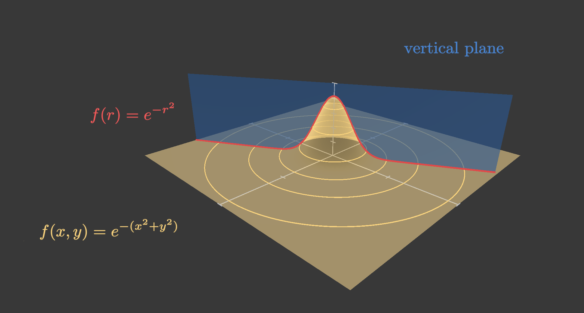
The function \(f_2(r)\) describes a smooth, bell-shaped surface above the \(xy\)-plane, shown in yellow in the image above. As already discussed the surface has perfect rotational symmetry indicated by the circular contours. That means any vertical cross-section through the origin produces the same curve. In particular, the cross-section along the \(x\)-axis (where \(y = 0\)) reduces to our familiar one-dimensional case \(e^{-x^2}\). Because this symmetry holds in all directions, we can generalize this reduction to \(e^{-x^2}\) and write \(e^{-r^2}\) for the equation of all intersection curves.
Let us now try to solve the 2-dimensional integral that means we have to determine the volume under this 2-dimensional surface given by \(f_2\). We can use the approach with \(r\) by trying to solve this from a polar coordinates perspective.
We are going to consider thin walls of cylinders under the functions. The surface area of such an cylinder can be easily determined when flatten the cylinder out. Calculating the area of the so received rectangle we get the circumfrence of the circle of the cylinder, which is \(2\pi r\) times the height, which is the function evaluated at this radius, so \(e^{-r^2}\).
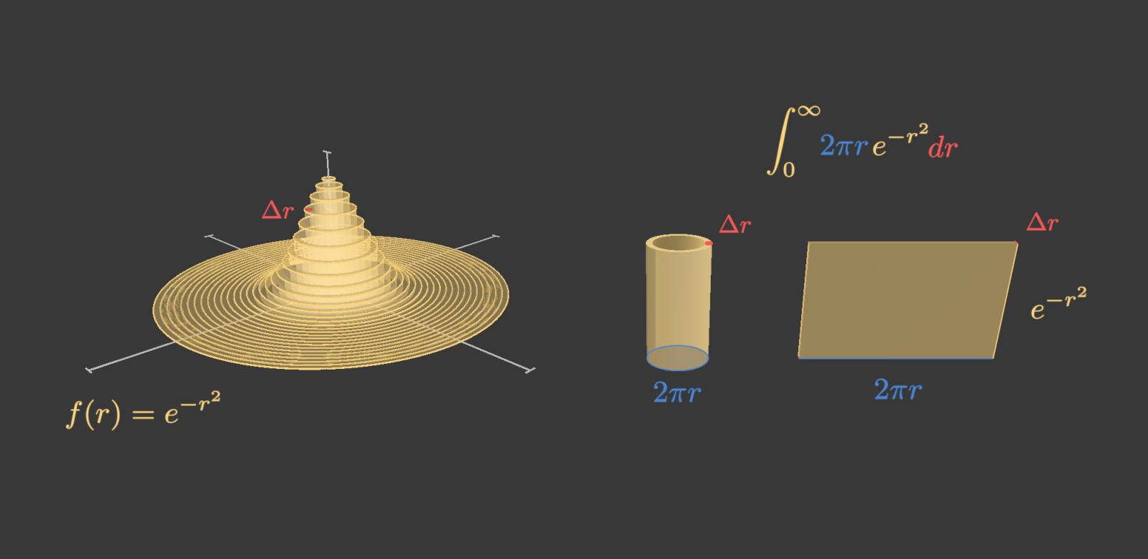
If we want to compute the whole volume under the function we can just add a tiny thickness \(\Delta r\) to that wall of that cylinder. Then the volume of one such cylinder wall will be (approximately but more and more accurate the smaller this \(\Delta r\) becomes) given by \(2\pi r e^{-r^2} \Delta r\) and the sum of all cylinder walls will yield approximately the total volume. If we let this \(\Delta r\) converge towards 0 then the sum will converge towards the exact total volume and we can write this as the following integral
\begin{equation} \int_{0}^{\infty} 2\pi r e^{-r^2} dr. \end{equation}The question is, are we now able to solve this integral? At a first glance not much seems to have changed — a nasty term of \(e^{-r^2}\) is still present. However, notice that the \(2r\) term is exactly the inner derivative of the exponential. So the anti derivative of the integral term will just be \(-e^{-r^2}\). Realizing that we can compute the integral by evaluatign at the boundaries leading to
\begin{equation} \pi \int_{0}^{\infty} 2 r e^{-r^2} dr = \pi [-e^{-\infty^2} - (-e^{-0^2})] = \pi \cdot 1 \end{equation}To be fully rigors here, for the upper limit of \(\infty\), we would consider input values of \(-e^{-r^2}\) diverging to \(\infty\) and we would see that the resulting values would converge towards 0.
And there it is — \(\pi\) appears quite naturally, just as one might suspect when dealing with rotational symmetry and sums of squares. Now, what does this tell us about the original one-dimensional case?
Recall that we started with the product \(e^{-x^2} e^{-y^2}\) and found that
\begin{equation} \int_{-\infty}^{\infty} \int_{-\infty}^{\infty} e^{-x^2} e^{-y^2} , dx , dy = \pi. \end{equation}However, since we are able to fully seperate the terms of involving \(x\) from those involving \(y\), we could have also considered the following integrals:
\begin{equation} \int_{-\infty}^{\infty} e^{-x^2} dx \int_{-\infty}^{\infty} e^{-y^2} dy = \pi. \end{equation}Both integrals are identical and both are exactly the integral we want to solve for. If we denote their value by \(I\), we have
\begin{equation} I^2 = \pi \quad \Rightarrow \quad I = \sqrt{\pi}. \end{equation}Obviously, the negative solution of the square root can be trivially ruled out.
And that is how Laplace was able to determine the normalization constant. To generalize the solution for the more general case \(e^{-h^2 x^2}\), we apply a simple change of variables \(x' = h x\), from which it follows \(dx' = h \, dx\). Hence, the solution to the integral in this case becomes
\begin{equation} I_{\text{generalized}} = \frac{\sqrt{\pi}}{h}. \end{equation}Putting everything together, we can now normalize the error curve so that its total area equals 1 — as required for any probability density function. We arrive at:
\begin{equation} f(x) = \frac{h}{\sqrt{\pi}}e^{-hh x^2}. \end{equation}This uses Gauss's original notation with his parameter \(h\). Using the modern convention, where \(\sigma^2 = \frac{1}{2h^2}\), the function becomes
\begin{equation} f(x) = \frac{1}{\sqrt{2\sigma^2\pi}}e^{-x^2/(2\sigma^2)}. \end{equation}Estimating parameters of normally distributed observations
We have seen how Gauss arrived at his distribution for random errors. Let us now return to the estimation of orbital parameters. How did Gauss use this information about the distribution of random errors to obtain the best estimates for those parameters?
Remember, we are in an overdetermined setting, as Gauss denoted by \(\mu > v\): there are more observations than unknown parameters. Let the functions that map the \(v\) parameters to the observed quantities be \(V_1,\dots,V_{\mu}\). For each such function we have a corresponding observation \(M_i\). This gives us the following overdetermined system:
\(M_1 = V_1(\text{\(v\) parameters})\)
\(M_2 = V_2(\text{\(v\) parameters})\)
\(\dots\)
\(M_{\mu} = V_{\mu}(\text{\(v\) parameters})\).
This system would have an exact solution only if all observations were completely free of error — which as already discussed, in practice, never happens. The data are inevitably riddled with random errors. Thus, any estimate of the parameters, say \(\hat{v}\), produces predictions \(V_i(\hat{v})\) that will not match the observations \(M_i\) exactly. There will be differences for almost all — and typically all — observations.
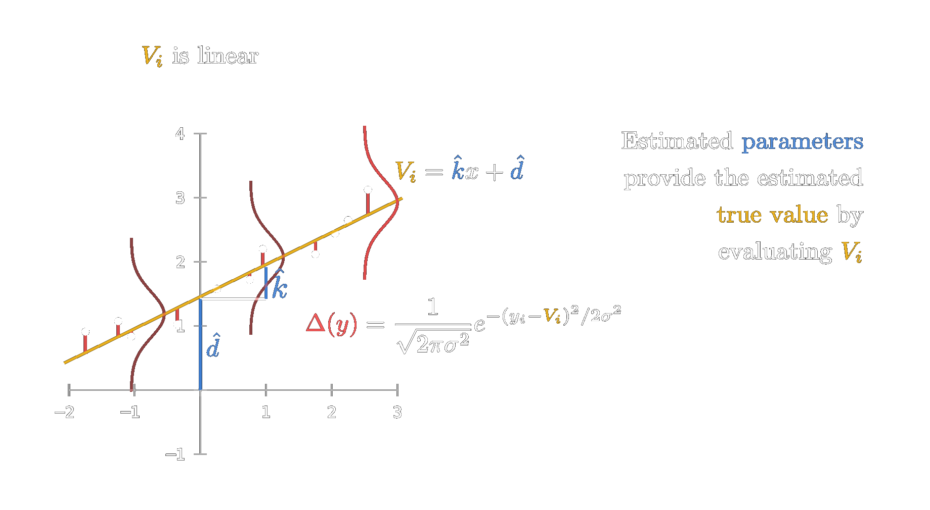
In the figure above, we see a function \(V_i\) determined by an estimated solution for the parameters \(\hat{v}\). If \(V_i\) is a linear function, as shown here, those parameters could for example be the slope \(k\) and the intercept \(d\). An estimated solution would then correspond to specific numerical values — for example, \(\hat{k} = 0.52\) and \(\hat{d} = 1.42\). In the case of orbit determination, the function \(V_i\) would of course not be a simple linear function but a more complex non-linear one describing the relationship between the six orbital parameters and one of the observed quantities, such as the ecliptic longitude of the celestial body.
Since the observations are affected by random errors and we are dealing with an overdetermined system, it is impossible to find an exact solution that fits all the data points. In the figure above, this means that the measurement errors cause the observations to scatter — they no longer fall perfectly on a single straight line. As a result, no single line can pass through every point exactly. Any solution to the system of equations will therefore leave small differences, or residuals, between the observed values and the model predictions, shown as the red gaps in the image.
However, the crucial question remains: how should we estimate the parameters \(v\) in the best possible way?
We have made this astonishing accomplishment and found the exact distribution of those random errors. However, how does this help us?
One possible approach is the following: given the probability distribution of the random errors, we want to choose the parameters \(v\) such that the observed data have the highest likelihood.
What does this mean? Since we know the probability distribution, we can determine the likelihood of an observation occurring at a certain distance from the true value. If we have a set of parameters, this ideally gives us the true value through the function \(V_i\). Based on the difference between the value predicted by \(V_i\) and the actual observation, we can calculate how likely that observation would be if the function truly represented the underlying value (see image above).
Therefore, we should choose the function — or equivalently, estimate the parameters — in such a way that the probability of obtaining the observed data is maximized. If we assume that each observation is drawn independently, we can compute the total probability of the entire set of observations simply by multiplying their individual probabilities. This leads to
\begin{equation} L(M) = \prod_{i=0}^{\mu} P(M_i|\hat{v}). \end{equation}Needless to say we can easily assign an exact expression to this Probability \(P\) because we derived the distribution before. We just have to use the difference from the function \(V\) to the observation as the input for the probability density function of the normal distribution and so we get
\begin{equation} P(M_i|\hat{v}) = \frac{1}{\sqrt{2 \pi \sigma^2}} e ^ {-(x_i-V_i(\hat{v})/\sigma)^2}. \end{equation}Again for the overall probability of all observations this gives us
\begin{equation} L(M) = \prod_{i=0}^{\mu} \frac{1}{\sqrt{2 \pi \sigma^2}} e ^ {-(x_i-V_i(\hat{v})/\sigma)^2}. \end{equation}Now, all that remains is to find the parameters \(\hat{v}\) such that this probability is maximized. At first, this might seem like a rather cumbersome task, since the parameters are buried deeply within the expression. However, let us start and see how far we can simplify it.
First, we can eliminate the product by taking the logarithm of the expression. This step is valid because the logarithm is a strictly monotonic function, meaning it preserves the location of the maximum. In other words, the parameter values that maximize the original expression will also maximize its logarithm. Doing that we get
\begin{equation} \sum_{i=0}^{\mu} \log\!\left(\frac{1}{\sqrt{2 \pi \sigma^2}} e^{-\frac{(x_i - V_i(\hat{v}))^2}{2\sigma^2}}\right). \end{equation}By applying the logarithm, we can also eliminate the exponential expression. Let us first separate the constant multiplicative factor in front of the exponential. The product becomes a sum of logarithms, and since the constant factor is the same for each term, it will simply multiply by \(\mu\). Thus, we obtain
\begin{equation} \mu \log\!\left(\frac{1}{\sqrt{2 \pi \sigma^2}}\right) + \sum_{i=0}^{\mu} \log\!\left(e^{-\frac{(x_i - V_i(\hat{v}))^2}{2\sigma^2}}\right). \end{equation}The first term is constant with respect to the parameters, so it can be ignored when finding the maximum. In the second term, the logarithm cancels the exponential, leaving us with
\begin{equation} -\frac{1}{2\sigma^2} \sum_{i=0}^{\mu} (x_i - V_i(\hat{v}))^2. \end{equation}The constant factor \(-\frac{1}{2\sigma^2}\) can again be ignored as it does not affect the location of the maximum. Also we can get rid of the negative sign by considering the minmum. Maximizing the negative of a sum is the same as minimzing the actual sum. This finally leads us to
\begin{equation} \sum_{i=0}^{\mu} (x_i - V_i(\hat{v}))^2. \end{equation}What have we just discovered? We have found that, in order to choose the parameters \(\hat{v}\) that maximize the likelihood of the observed data, we must minimize the sum above — that is, the sum of squared deviations between the observations and the model predictions. Returning to our geometric interpretation, the parameters \(v\), which define the shape of the function \(V\), must be chosen so that the sum of the squared red differences is as small as possible.
This approach of deriving an estimation for the parameters is known under the name maximum likelihood. For the normal distribution this yields the minimization of the sum of squares. For now we only have this general minimzation constraint. To get a formula that spits out the estimated paramters given the set of functions and the observations some additional work has to be done.
Generally speaking, a generalized analytical solution can only be achieved in the case where each \(V_i\) depends linearly on the parameters \(v\). So in case all \(V_i\) are linear functions, this minimization problem can be solved directly. Writing all observations and model functions in matrix form gives the familiar expression
\begin{equation} \mathbf{M} = \mathbf{V} \mathbf{v} + \boldsymbol{\epsilon}, \end{equation}where \(\mathbf{M}\) is the vector of measured values, \(\mathbf{V}\) contains the coefficients that describe how each parameter influences the observations, so in other words that is the linear map where each line corresponds to a linear function \(V_i\). The \(\boldsymbol{\epsilon}\) represents the random errors. The goal is to find the vector of parameters \(\hat{\mathbf{v}}\) that minimizes the sum of squared differences between the predicted values by the functions and the observations, so \(\|\mathbf{M} - \mathbf{V}\mathbf{v}\|^2\). By setting the derivative of this expression with respect to \(\mathbf{v}\) to zero, we obtain the so-called normal equations:
\begin{equation} \mathbf{V}^T \mathbf{V}\, \hat{\mathbf{v}} = \mathbf{V}^T \mathbf{M}. \end{equation}Solving this system yields the estimate of the parameters. This method of estimating the paramters is called the method of least squares.
When the functions \(V_i\) depend nonlinearly on the parameters, things are not as straightforward. In that case, the expression to be minimized can no longer be solved analytically (at least in most cases). However, the same principle still applies: we seek the parameters that minimize the sum of squared residuals. The practical way to do this is to start from an initial guess \(\hat{v}_0\), linearize the functions \(V_i\) around that point, and then iteratively adjust the parameters in the direction that reduces the residuals — a process guided by the derivatives (or gradients) of \(V_i\) with respect to the parameters.
The iterative procedure repeatedly updates the parameter estimates until the changes become negligibly small. In essence, it extends Gauss's elegant idea to cases where the dependence between observations and parameters cannot be expressed as a simple line by iteratively following the gradient. This procedure for solving optimization problems is very useful and is usually referred to as gradient descent. The whole methodology for non linear functions of least squares is usually called nonlinear least squares.
Using this method of least squares Gauss was able to estimate orbital parameters with astonishing precision. In particular, as Giuseppe Piazzi discovered the minor planet Ceres he could only observe it for about 40 days before it disappeared behind the Sun. Because of this short observation period, other astronomers could not predict where it would reappear in the sky months later. Ceres is very faint celestial object and shows no diameter like other bigger planets. So the only difference from the surrounding stars is the movement, which makes it very hard to identify. Thus back at the times many thought Ceres might be lost forever.
However, with just 24 years old, Gauss applied his new mathematical approach — this method of least squares with the underlying normal distribution as the distribtion for random errors — to compute the most probable orbit of Ceres from the limited, noisy data available. When Heinrich Olbers looked in the region Gauss predicted (at the end of 1801 and start of 1802), Ceres was found almost exactly where Gauss said it would be. This was a stunning success — it validated Gauss's method and indicated that the error curve of \(e^{-x^2}\) for random errors might be indeed correct.
But why is the normal distribution so important?
We have now explored Gauss's approach to the normal distribution in detail and have seen that it found immediate application in the estimation of orbital parameters. But why are random errors actually distributed according to this probability density function? And why does the normal distribution play such a central role — why is it so often assumed as the default case whenever no other information about a distribution is available?
We have already seen that with only a few, almost trivial assumptions — essentially just that the empirical mean is the best estimator is debatable — one is immediately led to this and only this distribution. There is, however, another route: when we consider the problem in multiple dimensions, a set of very mild assumptions again leads uniquely to the normal distribution. Let us take a closer look at this derivation.
Herschel-Maxwell Derivation
Assume we have a target in a two-dimensional setting. This could be, for instance, a dartboard, or an astronomical object we aim to center in a telescope's crosshairs. We make several attempts and thus obtain a collection of observations. What is the distribution of these aiming errors?
At first glance, this seems to require much more information — surely, from such a general description, no specific functional form for the distribution can be deduced? Surprisingly, only two assumptions — both of which most people would accept without hesitation — are again sufficient to leave the normal distribution as the only possible solution.
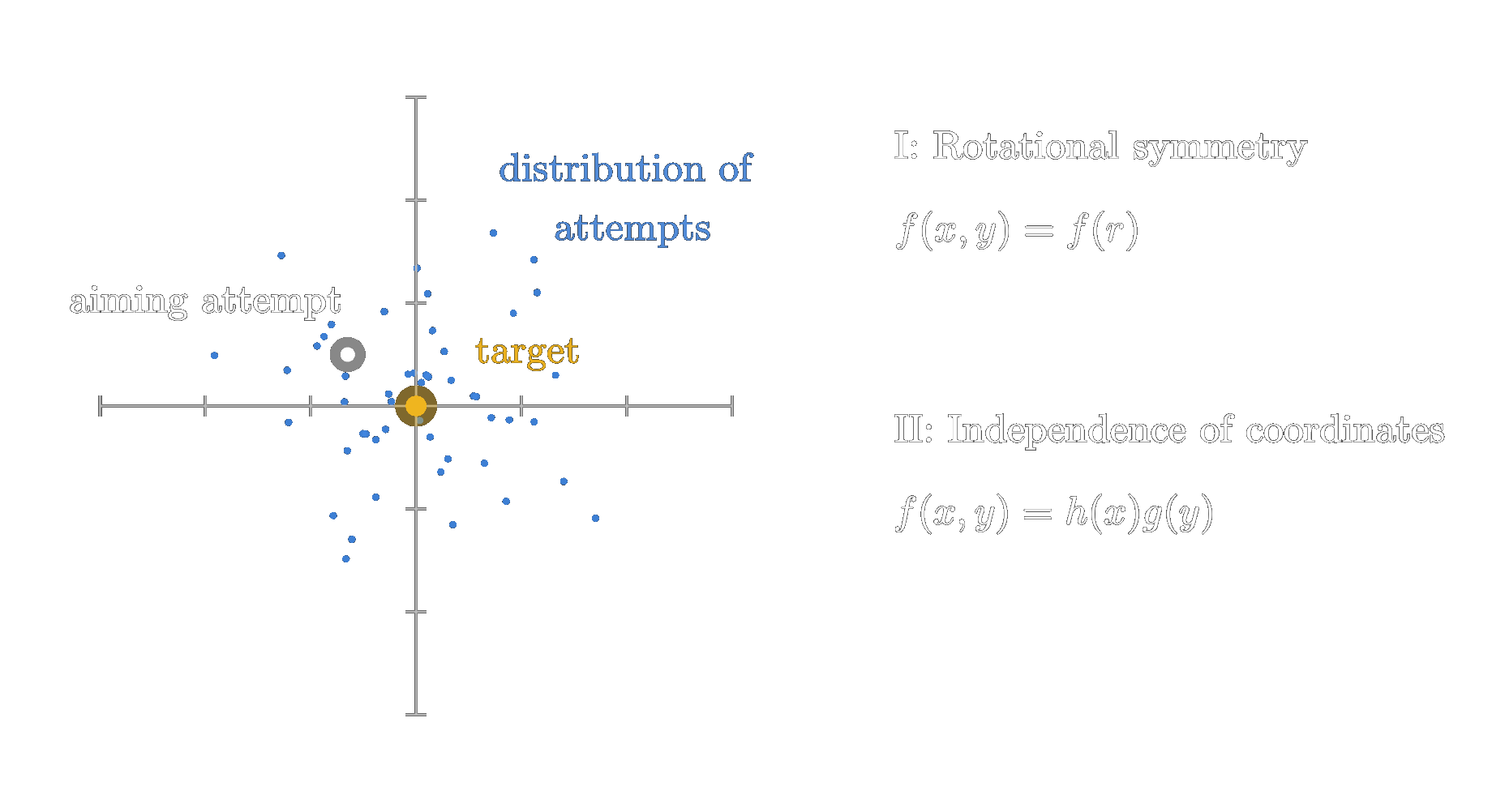
The first assumption is rotational symmetry: the distribution depends only on the distance from the center (the radius), not on the direction. Thus we can write
\begin{equation} f(x, y) = f(r). \end{equation}The second assumption is independence of the coordinates: knowing the \(x\)-coordinate of a shot tells us nothing about its \(y\)-coordinate. In terms of the probability density function, this means it can be expressed as the product of two functions, each depending only on one coordinate:
\begin{equation} f(x, y) = h(x) g(y). \end{equation}Both assumptions appear completely harmless, yet the only distribution that satisfies them simultaneously is the two-dimensional normal distribution. Of course, this argument generalizes naturally to higher dimensions, where the only solution is the \(n\)-dimensional normal distribution.
Let us see why this is the case. Due to the first assumption — rotational symmetry — the second assumption \(f(x, y) = h(x) g(y)\) can be restricted further. Since we can rotate the coordinate system by \(90^\circ\), the two functions must in fact be identical, hence
\begin{equation} f(x, y) = h(x) h(y). \end{equation}Furthermore, consider a point at distance \(r\) from the center. Because of rotational symmetry, we can always rotate this point onto one of the coordinate axes, leading to
\begin{equation} f(r) = h(r) h(0). \end{equation}This implies that \(h\) differs from \(f\) only by a constant factor, so we can write
\begin{equation} f(r) = f(\sqrt{x^2 + y^2}) = c f(x) f(y), \quad c \in \mathbb{R}. \end{equation}To avoid the square root, we can define a new function \(F(x) = f(\sqrt{x})\). Then the condition becomes
\begin{equation} F(x^2 + y^2) = c F(x^2) F(y^2), \quad c \in \mathbb{R}. \end{equation}Since this must hold for arbitrary \(x^2\) and \(y^2\), it must also generalize to any number of terms, for example,
\begin{equation} F(x_1^2 + x_2^2 + x_3^2) = c_1 F(x_1^2 + x_2^2) F(x_3^2) = c_1 c_2 F(x_1^2) F(x_2^2) F(x_3^2). \end{equation}In general, we can therefore write
\begin{equation} F\!\left(\sum_i x_i\right) = c \prod_i F(x_i), \quad c \in \mathbb{R}. \end{equation}Now consider \(x_i \in \mathbb{N}\). It can easily be shown that this implies
\begin{equation} F(n) = c F(1)^n = c b^n, \quad c, b \in \mathbb{R}. \end{equation}The same holds for rational numbers. Assuming \(F\) is continuous, this extends naturally to all real numbers:
\begin{equation} F(x) = c b^x, \quad c, b \in \mathbb{R}. \end{equation}The solution to this functional equation is therefore the exponential function. For our original function \(f(x)\), we thus obtain
\begin{equation} f(x) = c b^{x^2}, \quad c, b \in \mathbb{R}. \end{equation}Introducing the natural base \(e\), and writing in terms of the radius \(r\) we can rewrite this as
\begin{equation} f(r) = c e^{k r^2}, \quad c, b \in \mathbb{R} \quad k \in \mathbb{R}^-, \end{equation}where we restrict \(k\) to negative real values, following the same reasoning as in the previous section — because otherwise the function would diverge and could not represent a probability density. The constant \(c\), as we have already seen, must include the term involving \(\pi\) to ensure that the probability density function is properly normalized.
This result is quite remarkable. It shows, among other things, why the appearance of the constant \(\pi\) in the normal distribution arises so naturally: a distribution describing purely random errors — essentially pure noise — should, of course, be rotationally symmetric. It also explains why the argument involves \(x^2\) rather than \(x\): this quadratic dependence guarantees rotational symmetry.
Nevertheless, the deeper question remains: why does this distribution appear so universally? Gauss's own derivation sheds further light on the matter, yet even that does not completely resolve the mystery. His reasoning still feels, in parts, a little too much like a hand-waving argument.
The normal distribution as the central limiting function
Long before the time of Gauss, it was already known that the binomial distribution converges to the same characteristic shape — regardless of whether the probability of success was evenly balanced, as in a fair coin toss with 50/50 odds, or more biased, such as 90/10. De Moivre, as early as 1733, had already derived the exact expression of the limiting distribution of the binomial law. Once again, it was the familiar curve of the form \(e^{-x^2}\).
In modern notation, the binomial distribution with parameters \(n\) and \(p\) can be approximated by the normal distribution
\begin{equation} B(n, p) \approx \mathcal{N}(np, np(1 - p)). \end{equation}The binomial distribution represents the sum of \(n\) Bernoulli trials, each taking the values 0 or 1 — for example, \(n\) consecutive coin flips. What is remarkable, however, is that this convergence towards the normal distribution is not limited to random variables that follow a Bernoulli distribution.
In fact, the sum of a large number of independent random variables, each with finite variance, will always tend to follow a normal distribution, regardless of the form of the individual underlying distributions.
\begin{equation} \frac{\sum_{i=1}^{n} X_i - n\mu}{\sqrt{n\sigma^2}} \xrightarrow[n \to \infty]{d} \mathcal{N}(0,1). \end{equation}This result is known as the Central Limit Theorem and provides a profound explanation for why the normal distribution appears so frequently in nature and in measurement data. Most quantities we observe are the outcome of many small, independent random effects, each contributing only a tiny amount to the total result. The accumulation of these influences inevitably gives rise to the familiar bell-shaped curve.
Thus, while Gauss's intuitive and functional reasoning hinted at the special role of the normal distribution, the Central Limit Theorem ultimately reveals probably the more broader reason why it is so universal. Although the property of rotational symmetry while keeping independence in the coordinates in Maxwell's/Herschel's derivation makes the normal distribution already quite normal and would definitely make an argument on its own why we would encoutner this distribution in nature all over the place.
However the Central Limit Theorem also is more an argument of symmetry. When it comes to sums of random variables, there exists a distribution that is invariant regarding the summation. Let us have a more detailed look at this.
The normal distribution as the stationary point of convolutions
An interesting way to view the Central Limit Theorem is through the concept of convolutions. In probability theory, the sum of two independent random variables corresponds to the convolution of their respective probability density functions. Repeatedly adding independent random variables therefore means performing repeated convolutions of their distributions.
As this process continues — as we convolve more and more distributions — the resulting function becomes progressively smoother and appears to approach a stable, universal form.
In fact, by working through the details, one can show that all distributions converge toward a single universal shape under repeated convolution.
Naturally, this raises the question: what is that shape? If we could find a distribution that remains unchanged under repeated convolution, we would have identified the fixed point of this process.
Remarkably, this limiting, stationary form is again the shape described by \(e^{-x^2}\) — that is, the shape of the normal distribution.
Mathematically, if \(f(x)\) and \(g(x)\) are two independent probability densities, then the distribution of their sum is given by
\begin{equation} (f * g)(x) = \int_{-\infty}^{\infty} f(t) \, g(x - t) \, dt. \end{equation}The normal distribution is unique in that it remains invariant under this operation — that is, the convolution of two normal distributions yields another normal distribution (with appropriately added variances). This property identifies it as the stationary point of the convolution process.
In this sense, the Central Limit Theorem can be understood as describing a kind of attractor behavior: as independent random effects combine, the resulting distribution is drawn closer and closer to the normal law, regardless of the original form of the individual distributions.
This interpretation beautifully illustrates how random errors that result from the combination of many different random effects naturally tend to follow a distribution similar in shape to the normal distribution. The more different effects overlap the more it will approach the shape of a normal distribution.
Conclusion
Huh, that was quite a lot — and certainly one of the longest Stories in our database. Yet the normal distribution truly deserves this space — it sits at the very heart of mathematics, it dominants the field of probability theory and it kind of is the fundamental perception of continous randomness itself. And to be fair, there is still so much more that could be said. The normal distribution is one of those topics you could wander through for weeks, always discovering something new, always feeling that a deeper connection lies just beneath the surface.
However, we already got a lot to know this time. We started by examining how Gauss originally arrived at it — saw how a very limited set of assumptions already fixes the equation of the distribition of random errors to the exact form of \(e^{-x^2}\). We then were able to use this equation about random errors to estimate parameters from observations. We saw how back at the time this emmidiately found great usage in the estimation of orbital parameters.
Putting this historical approach into the broader context of why there exists something like the normal distribution led us to a whole new understanding of the normal distribution and how it relates to all the constants involved in its equation. We were able to deduce a very profound understanding and intuitive feeling for why \(\pi\) so naturally shows up in the formula — the square numbers ensure rotational symmetry (a property obviously required for the distribution of random errors / pure noise) and there \(\pi\) is usually not far away. The number \(e\) also comes very naturally. It essentially comes from the fact that when you consider multiple outcomes, you multiply their probabilities — and the exponential function once again preserves rotational symmetry in higher dimensions as it turns summation into multiplication, turning the sum of squares into the multiplication of independent probabilities.
After reading this Story, seeing the formula of the normal distribution feels like a completely different experience. You can truly sense how every single part of it flows naturally from the vast landscape of mathematics — all converging beautifully into this thing we call the normal distribution, as it really is the normal, the default, distribution, uniquely holding rotational symmetry for independend random variables and acting as the attractor for sums of independent random variables.
And with those beautiful words, we will leave it here for now...