Introduction
Since the days of Pascal and Fermat — and at the very latest since Jakob Bernoulli's Ars Conjectandi, published posthumously in 1713 — it was known how to determine the probabilities for something like \(n\) consecutive fair coin tosses. The equation of the so-called binomial distribution
\begin{equation} P(k) = \binom{n}{k}\frac{1}{2^n} \end{equation}yields the exact probability of getting \(k\) heads in \(n\) tosses. (For an event with chance \(p\) instead of \(\tfrac{1}{2}\) it reads \(\binom{n}{k}p^k(1-p)^{n-k}\), but let us stick to the fair coin for now — just like de Moivre did for most of his journey.) So questions like, for example, what is the probability that I get at least 7 heads out of 10 tosses could be easily answered by just summing up the corresponding results of the above equation:
\begin{equation} \frac{\binom{10}{7} + \binom{10}{8} + \binom{10}{9} + \binom{10}{10}}{2^{10}} = \frac{120 + 45 + 10 + 1}{1024} = \frac{176}{1024} \approx 17.2\%. \end{equation}However, try the same with 3600 tosses — an example de Moivre himself used — and ask for the probability that the number of heads lands somewhere between 1770 and 1830. Now you have to sum up 61 terms, and every single one of them contains a binomial coefficient of monstrous size: \(\binom{3600}{1800}\) alone has 1082 digits. By hand — with quill and ink. A hopeless endeavor.
So there was clearly a need for a way around this — if not for practical purposes, then at least for sharpening results like Bernoulli's law of large numbers. Which brings us to the man of this story. Abraham de Moivre was born in 1667 in Vitry, in the Champagne, into a Protestant family. When Louis XIV revoked the Edict of Nantes in 1685, life became dangerous for French Protestants — de Moivre was reportedly imprisoned for a while — and he ended up in London, where he stayed for the rest of his life. He was a Fellow of the Royal Society since 1697 and a friend of Halley and Newton, but he never got a university position. Instead, he made his living as a private tutor and by solving problems of chance for wealthy patrons and gamblers — allegedly from a table at Slaughter's Coffee House in St Martin's Lane. Newton himself is said to have sent people who came to him with such questions away with the words: "Go to Mr. de Moivre; he knows these things better than I do."
In November 1733 de Moivre handed some friends a short Latin paper of seven pages, titled Approximatio ad Summam Terminorum Binomii \((a+b)^n\) in Seriem expansi — an approximation of the sum of the terms of the binomial \((a+b)^n\) expanded into a series. Only two copies are known to have survived. Five years later he included his own English translation in the second edition of his Doctrine of Chances (1738, pages 235–243). These few pages mark the very first encounter with the normal curve in history.
The actual derivations, however, are scattered over his Miscellanea Analytica of 1730, the just mentioned supplement Approximatio, a letter he received from James Stirling, as well as Stirling's Methodus Differentialis. So this story will collect all those pieces and try to walk the actual path of discovery alongside de Moivre (and partly also Stirling).
The Basic Idea
It all started with a question. In 1721 a Scottish gentleman named Alexander Cuming — also a fellow of the Royal Society and a friend of de Moivre and Stirling — challenged de Moivre with a problem. It essentially asked: if you toss a coin \(n\) times, by how much does the number of heads deviate from the expected value \(\tfrac{n}{2}\) on average?
De Moivre found an exact answer, and it is a surprisingly neat one. We will skip the details here (maybe we will cover it in another story sometime) but essentially he found out that the average deviation is nothing but \(\tfrac{n}{2}\) times the middle term. So the whole question boils down to one single number: how big is the middle term of a binomial distribution when \(n\) is large? And that is how the middle term entered de Moivre's life. When he later wrote the Approximatio, he began with: "It is now a dozen years or more since I had found what follows", exactly dating back to 1721, and he even credited Alexander Cuming for motivating him to find an approximation for the middle term. So this whole endeavor of finding an approximation to the binomial distribution seems to have started right with that.
In any case, it certainly shaped, to some extent, how de Moivre approached the problem of approximating the binomial distribution. Working out an approximation for the middle term first has the advantage that you can then move on to the other terms fairly easily. The expression for any single term may contain huge products in the form of factorials, but the ratio of two neighboring terms is remarkably simple:
\begin{equation} \frac{\binom{n}{k+1}}{\binom{n}{k}} = \frac{n-k}{k+1}. \end{equation}So once you have an approximation for the middle term, you can easily work your way to the terms right next to it. The figure below shows this for the case \(n=20\). The largest term (which is the middle term when an event is just as likely to happen as not) is drawn in yellow. Starting from it, you can propagate term by term to the right (or to the left) simply by multiplying by a single factor each time.
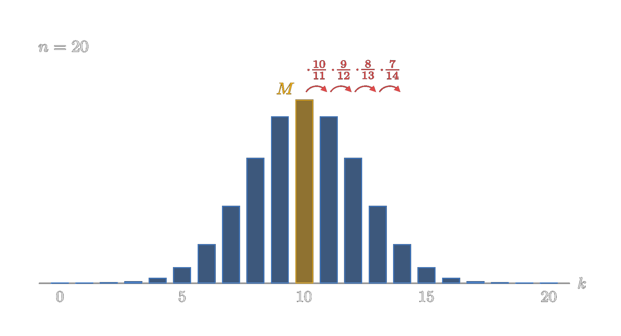
In short: the middle term fixes the height of the peak of the binomial distribution, and the propagation outward determines how the terms fall off. Find a simple approximation for both, and you have an approximation for the geometric shape of the distribution. Questions about specific probabilities, like the one from the beginning about getting between 1770 and 1830 heads, then turn into finding a certain portion of the area under this shape.
The middle term itself is given by
\begin{equation} \binom{2m}{m} = \frac{(2m)!}{m!\,m!}. \end{equation}As you can see, this term alone already contains large factorials (for large \(m\), or \(n\)) and is, in general, a huge product. The propagation factors pile up as well: for large \(m\) or \(n\) and a significant distance from the middle, they too grow into a sizable product.
It is therefore natural to continue the investigation in the logarithmic domain, and that is exactly what de Moivre did. Moreover, a few decades earlier Nicholas Mercator had published his famous series
\begin{equation} \ln(1+x) = x - \frac{x^2}{2} + \frac{x^3}{3} - \frac{x^4}{4} + \cdots, \end{equation}so by then the logarithm was no longer just a handy trick for evaluating large, unwieldy products. It had become a genuine object of analysis.
So de Moivre's plan was this: take the logarithm of everything, turn the products into sums, and then somehow simplify those sums, ideally by finding a simple approximation for them. This eventually should tame the enormous factorials involved and with that estimating the essence of the shape of the binomial distribution will be possible.
Stirling's Approximation
De Moivre had plenty experience with logarithms. His Miscellanea Analytica even contained a table of the (base-10) logarithms of \(10!, 20!, 30!, \dots\) all the way up to \(900!\), given to fourteen figures. He had computed it the honest and hard way, by adding up logarithms one after another. However, as might be expected with such lengthy, cumbersome calculations that was exactly where a mistake happened. So, a few days after the book was out, a letter from James Stirling arrived — the very same Stirling by the way we met in the story Stirling Numbers — The Second Kind. Stirling pointed out that the table was wrong from the fifth decimal on. As it turns out, a slip in the very first entry, \(\log 10!\), had simply been carried along through every entry below it (and two more slips further down did the same). But Stirling did not just complain: he added, without proof, an approximation for \(\log n!\) that contained an interesting constant of \(\log\sqrt{2\pi}\).
De Moivre had already found an approximation by himself, though unpublished and he could not figure out what the constant was — he had just determined it numerically. Delighted about what the constant turned out to be he included Stirling's contribution when he later published his own approximation series. Let us follow de Moivre's derivation here.
The first move is a clever rewriting. Write \(n!\) backwards as \(n(n-1)(n-2)\cdots 1\) and pull a factor \(n\) out of every single factor:
\begin{equation} n! = \prod_{k=0}^{n-1}(n-k) = n^n \prod_{k=1}^{n-1}\left(1-\frac{k}{n}\right) \qquad \Longrightarrow \qquad \log n! = n\log n + \sum_{k=1}^{n-1}\log\left(1-\frac{k}{n}\right). \end{equation}The factor for \(k=0\) is just 1, so it drops out. Now every logarithm in the sum over \(k\) is of the form \(\log(1-t)\) with \(t \lt 1\), so we can replace it by Mercator's series, \(-\log(1-t) = t + \tfrac{t^2}{2} + \tfrac{t^3}{3} + \dots\):
\begin{equation} \sum_{k=1}^{n-1}\log\left(1-\frac{k}{n}\right) = -\sum_{k=1}^{n-1}\sum_{p=1}^{\infty}\frac{1}{p}\frac{k^p}{n^p} \qquad S_p = 1^p + 2^p + \dots + (n-1)^p. \end{equation}Note that the term \(k^p\) actually represent the sum of powers, so for example, a series like \(1+4+9+16+\dots\). Well not quite since we first sum over \(p\) and then over \(k\). But if we swap the order of summation (allowed because we have absolut convergence here), we will get exactly that
\begin{equation} -\sum_{p=1}^{\infty}\sum_{k=1}^{n-1}\frac{1}{p}\frac{k^p}{n^p} = -\sum_{p=1}^{\infty}\frac{1}{p\,n^p}\,S_p, \qquad S_p = 1^p + 2^p + \dots + (n-1)^p. \end{equation}There they are, the sums of powers, which we denote here as \(S_p\). The reason for de Moivre trying here to isolate this sums of powers is that a general formula for them had just been found by Jakob Bernoulli a few years earlier (published in the Ars Conjectandi, 1713). Written in terms of \(N = n-1\), this general formula reads
\begin{equation} S_p = \frac{N^{p+1}}{p+1} + \frac{N^p}{2} + \frac{p}{12}N^{p-1} - \frac{p(p-1)(p-2)}{720}N^{p-3} + \dots, \end{equation}where the numbers \(\tfrac{1}{12}, -\tfrac{1}{720}, \dots\) contain what we today call the Bernoulli numbers.
That gives him something nice to work with. De Moivre continues by swaping again the order of summation, now with the newly introduced formula of Bernoulli. However, in order to not loose track of all that swapping, let's take a short pause and briefly visualize what we have done to the series so far and what the next step is. So, in the following image we have an abstracted visualization of the original series and the first change in the order of summation we just did.
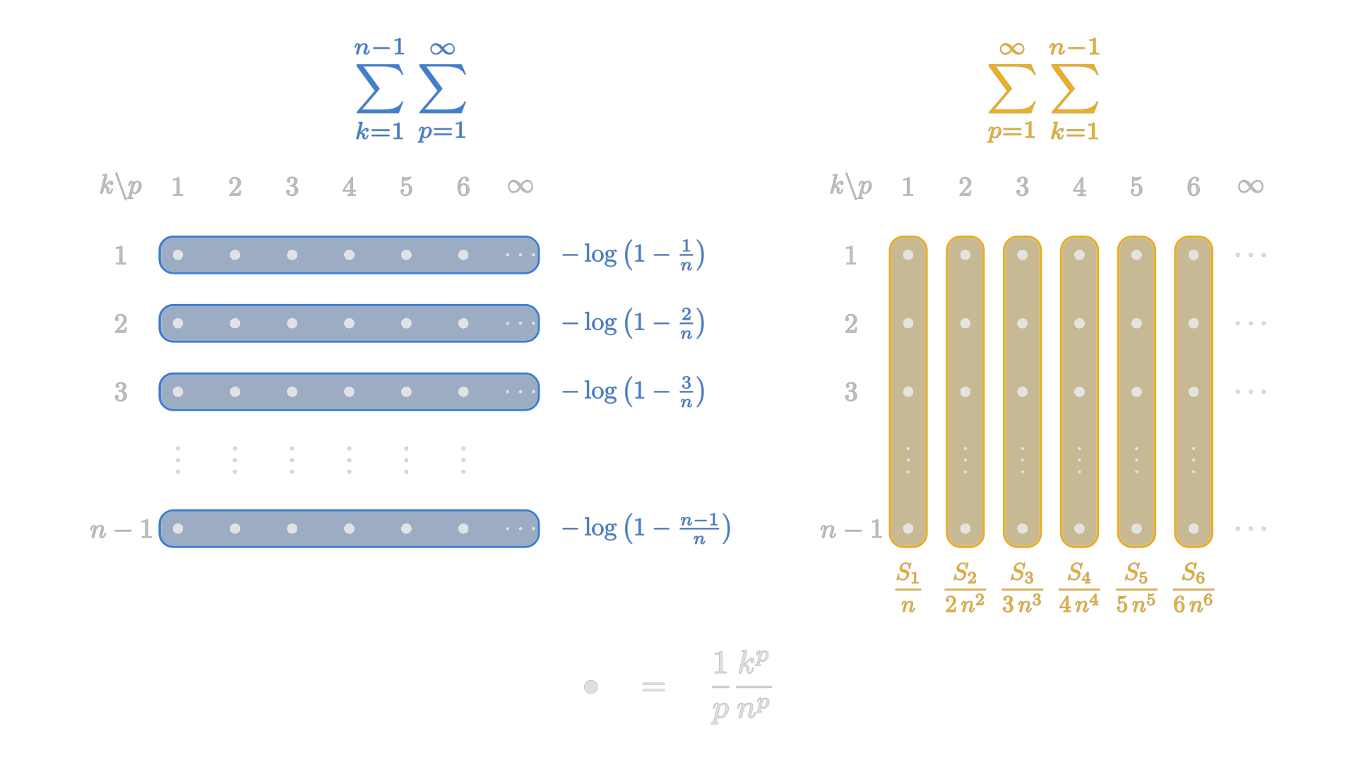
As we have already mentioned, the double series is absolute convergent. As long as we do not let \(n\rightarrow\infty\), there is anyway only one infinite sum in play, and its absolute convergence is easy to show (but even with \(n\rightarrow\infty\) we are fine). So summing along the columns instead of the rows, as shown in the image above is perfectly fine.
After replacing the sums of power by Bernoulli's closed formula, de Moivre, again, changes the order of summation. However, this time, that causes some issues. You see, we have now introduced Bernoulli's polynomial expression, that is itself a sum of terms, a finite series. However, finite, only for a fixed \(p\). But the summation over \(p\) is an infinite one.
Therefore, by looking at the following image, we see, Bernoulli's expression eventually will also include infinitely many terms as we move to the right, that is as we increase \(p\) towards infinity.
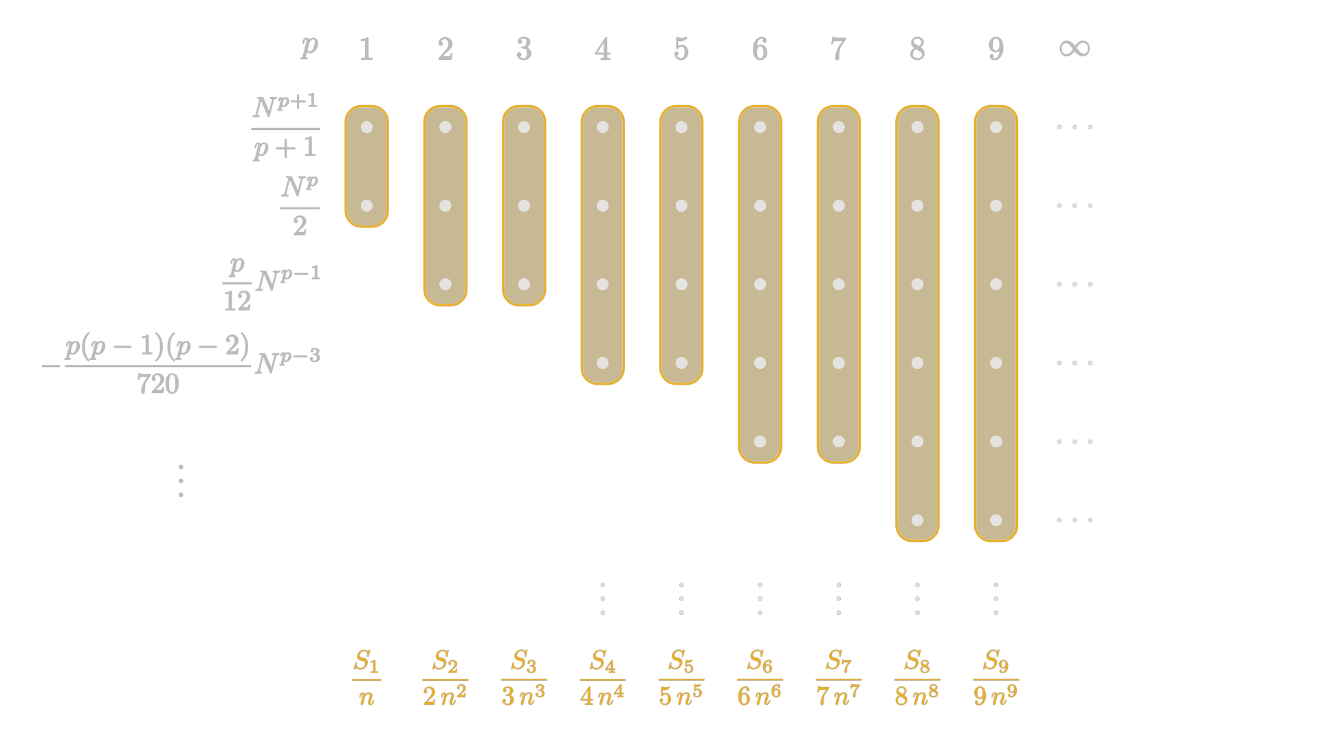
And Bernoulli's expression is an alternating series, whereby the indivdual terms keep increasing. That is not a big deal when evaluating the sum of a power sieres for a given power with it (because the terms nicely keep canceling out each other) — but it becomes an issue when all powers up to infinity are considered. To put things short: the given double series here is no longer absolute convergent. This implies that technically, we are not allowed to change the order of summation. De moivre, unaware of that, as such details were not known in his time, does so anyway and still arrives at a useful result.
However, as we will see at the end of this story, his (and also Stirling's as they are basically identical) new series for the logarithm of \(n!\) is actually only an assymptotical approximation and does eventually diverge. The modern approach, for avoiding all of that, would be to consider partial sums only, and then estimate the error leftover by an integral (or similar), which usually then leads to the Euler-Maclaurin equation.
Anyway, continuing with de Moivre's way, we change the order of summation, as visualized in the following image:
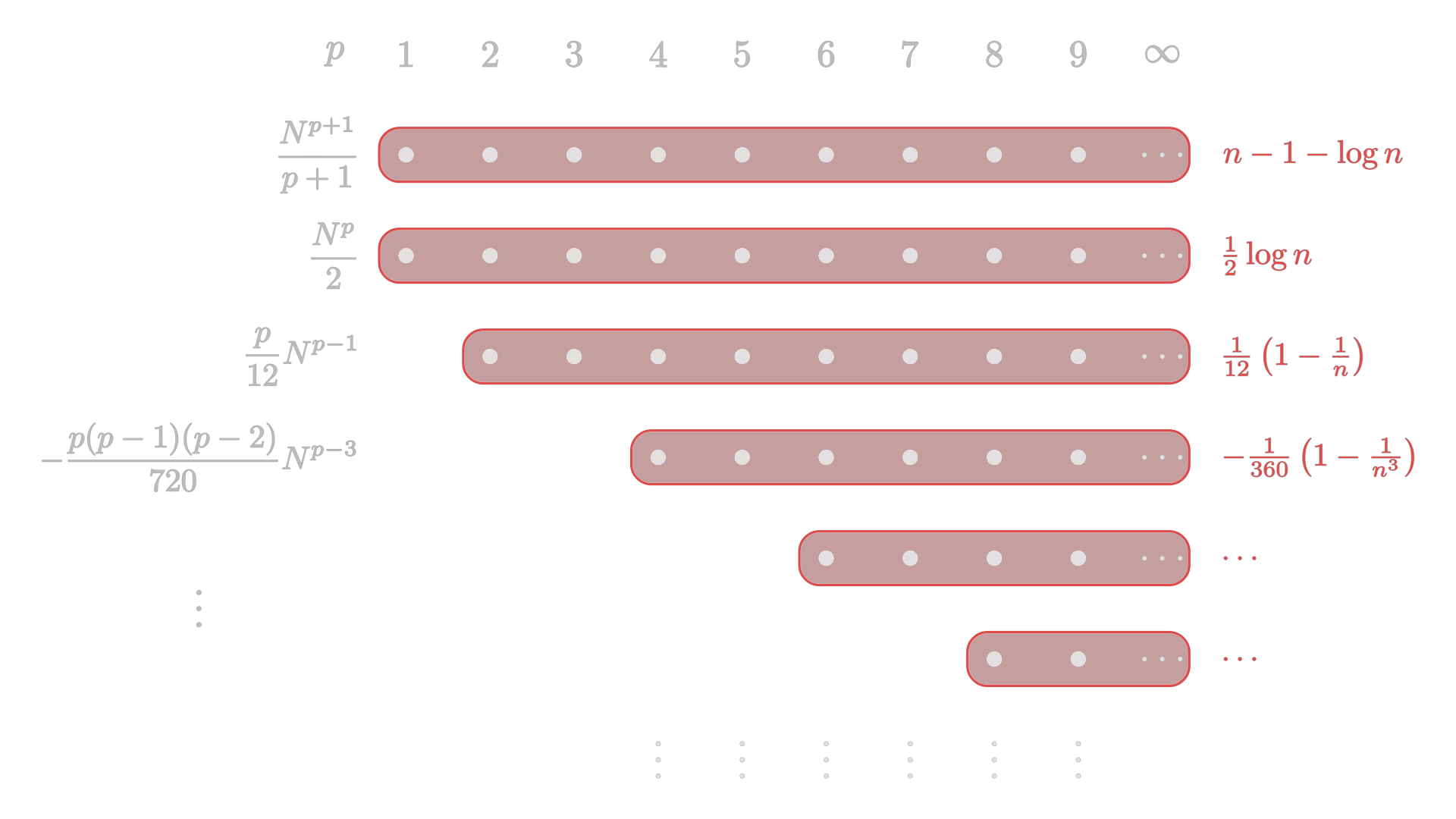
The summation is now the other way round. Instead of our Bernoulli formula being summed up over all \(p\), we now look at the sum of one single term of it over all \(p\), that is one row in the image above, and sum them up, line by line.
De Moivre does not actually write all of this down in a single line. Instead, he computes the sum for the first four terms of Bernoulli's formula, spots the pattern, and extrapolates it to all remaining terms.
To sum the first term, we can use \(\tfrac{1}{p(p+1)} = \tfrac{1}{p} - \tfrac{1}{p+1}\), and by introducing \(x=\frac{N}{n}\), we see that it is, in fact, Mercator's series again:
\begin{equation} \sum_{p=1}^{\infty}\frac{N^{p+1}}{p(p+1)\,n^p} = n\sum_{p=1}^{\infty}\left(\frac{x^{p+1}}{p} - \frac{x^{p+1}}{p+1}\right). \end{equation}For the first sum, we factor out \(x\) and see that it evaluates to \(-x\log(1-x)\). The second sum is simply missing the first term \(x\), so it equals \(-\log(1-x)-x\). Combining the results gives
\begin{equation} -nx\log(1-x)+n\log(1-x)+nx, \end{equation}which, after rewriting everything in terms of \(n\) (note that \(\log\left(\tfrac{1}{n}\right)=-\log(n)\)), simplifies to
\begin{equation} -\log n + n -1. \end{equation}The second term is up to a constant factor just Mercator's series itself:
\begin{equation} \sum_{p=1}^{\infty}\frac{N^p}{2p\,n^p} = \frac{1}{2}\sum_{p=1}^{\infty}\frac{x^p}{p} = -\frac{1}{2}\log(1-x) = \frac{1}{2}\log n. \end{equation}From the third term onward, the numerator contains at least one factor of \(p\), which cancels the \(p\) in the denominator, so logarithmic expressions no longer appear. For the third term, we are left with a plain geometric series (it starts at \(p = 2\) because for \(p = 1\), Bernoulli's formula has no such term):
\begin{equation} \sum_{p=2}^{\infty}\frac{1}{p\,n^p}\cdot\frac{p}{12}N^{p-1} = \frac{1}{12n}\sum_{p=2}^{\infty}x^{p-1} = \frac{1}{12n}\cdot\frac{x}{1-x} = \frac{1}{12}\left(1-\frac{1}{n}\right). \end{equation}The fourth term (it starts at \(p = 4\)) is quite similar, except that products of consecutive integers now appear in front of the powers of \(x\); here, it is a product of two consecutive integers. This hints at differentiation, and indeed it is easy to see that we are dealing with the geometric series differentiated twice, \(\sum_{q\ge 0}(q+1)(q+2)x^q = \tfrac{2}{(1-x)^3}\)
\begin{equation} -\sum_{p=4}^{\infty}\frac{1}{p\,n^p}\cdot\frac{p(p-1)(p-2)}{720}N^{p-3} = -\frac{1}{720\,n^3}\sum_{q=1}^{\infty}(q+1)(q+2)\,x^q = -\frac{2n^3 - 2}{720\,n^3} = -\frac{1}{360}\left(1-\frac{1}{n^3}\right). \end{equation}From there on, the pattern continues: each further term contains the next Bernoulli number together with a higher-order derivative of the geometric series and so the final result will be:
\begin{equation} \begin{aligned} \log n! &= n\log n - \left[(n-1-\log n) + \tfrac{1}{2}\log n + \tfrac{1}{12}\left(1-\tfrac{1}{n}\right) - \tfrac{1}{360}\left(1-\tfrac{1}{n^3}\right) + \dots\right] \\ &= \left(n+\tfrac{1}{2}\right)\log n - n + \underbrace{\left(1 - \tfrac{1}{12} + \tfrac{1}{360} - \tfrac{1}{1260} + \tfrac{1}{1680} - \dots\right)}_{=:\,C} + \frac{1}{12n} - \frac{1}{360n^3} + \dots \end{aligned} \end{equation}De Moivre collects all terms that do not depend on \(n\) into the constant \(C\), which yields the following final result:
\begin{equation} \log n! = \left(n+\tfrac{1}{2}\right)\log n - n + C + \sum_{k=1}^{\infty}\frac{B_{2k}}{2k(2k-1)}\,\frac{1}{n^{2k-1}}, \qquad C = 1 - \sum_{k=1}^{\infty}\frac{B_{2k}}{2k(2k-1)}, \end{equation}whereby \(B_{2k}\) denotes the corresponding Bernoulli number and the closed summation formula for \(C\) can easily be found by just evaluating the expression for \(n=1\).
The obvious question now, of course, is: what is \(C\)? De Moivre simply added up the first few terms. The partial sums wiggle around a value of roughly \(0.919\) — and then they run away. The Bernoulli numbers eventually grow faster than any power, so the series for \(C\) does not actually converge at all. De Moivre, however, did not notice this; he only knew the first handful of Bernoulli numbers anyway. He writes that he "perceiv'd that it converged but slowly", and since the result, as he put it, "answered my purpose tolerably well", he stopped there.
As pointed out at the beginning of this section, this whole series for \(\log n!\) is actually divergent. Swapping the order of summation caused both the series for \(C\) and the series of Bernoulli numbers with odd powers of \(n\) to blow up. Historically, it was Thomas Bayes who pointed out this divergence, in a letter published posthumously in 1763.
Nevertheless, the approximation is anything but useless. The series approximates \(\log n!\) asymptotically. By this we mean the following: if we stop after a fixed number of terms, the error becomes arbitrarily small as \(n\) grows — in fact, it is always smaller in absolute value than the first term we left out. For a fixed \(n\), on the other hand, adding more terms initially improves the approximation, but only up to a certain point. After that, the terms grow again and the partial sums swing back and forth ever more wildly. This is exactly where the illegitimate change in the order of summation shines through, and it is also why we have to fix the number of terms and let \(n\) tend to infinity, and not the other way round.
In practice, the trick is therefore to stop at the right moment, namely around the smallest term, which yields the most accurate result possible. For \(n = 1\), which is exactly the case of de Moivre's series for \(C\), the smallest Bernoulli term is already the fourth one, \(\tfrac{1}{1680}\). This is why his partial sums never got much more precise than \(0.919\).
And what exactly is \(C\)? This is the part Stirling had figured out: he showed that \(C = \log\sqrt{2\pi}\). As mentioned at the beginning, Stirling had in fact also found an approximation for \(\log n!\). His series, essentially the same, looked a bit different though — it was written in powers of \(n + \tfrac{1}{2}\). When he published his derivation of in Methodus Differentialis a few years later, he shows how the approximation can be derivied in an even more elegant way. His derivation was based on more modern mathematics that included the Euler-Maclaurin series and is very close to what a modern derivation of today would look like. Hence we today call it Stirling's approximation, though the priority for the series is probably better assigned to de Moivre, as he had found it presumably already in the year 1721. The constant, though, definitely belongs to Stirling.
By the way, strictly speaking, what we usually mean by Stirling's approximation is
\begin{equation} n! \approx \sqrt{2\pi n}\left(\frac{n}{e}\right)^n, \end{equation}which is simply the leading part of the series above with \(C = \log\sqrt{2\pi}\), exponentiated to get rid of the logarithm.
For the sake of completeness, I want to briefly point out another more direct route to arrive at this result. It does not yield the whole approximation formula, only the first few terms again — so exactly the part we today refer to as Stirling's approximation — but it is a very visually pleasing derivation, and since this is Mathematics Visualized, it is definitely something we should not miss out on.
The idea is again to use the logarithm to turn the multiplication of the factorials into a more manageable sum
\begin{equation} \log n! = \sum_{i=1}^n \log i, \end{equation}and then to approximate the resulting discrete sum by an integral, as shown in the following image.
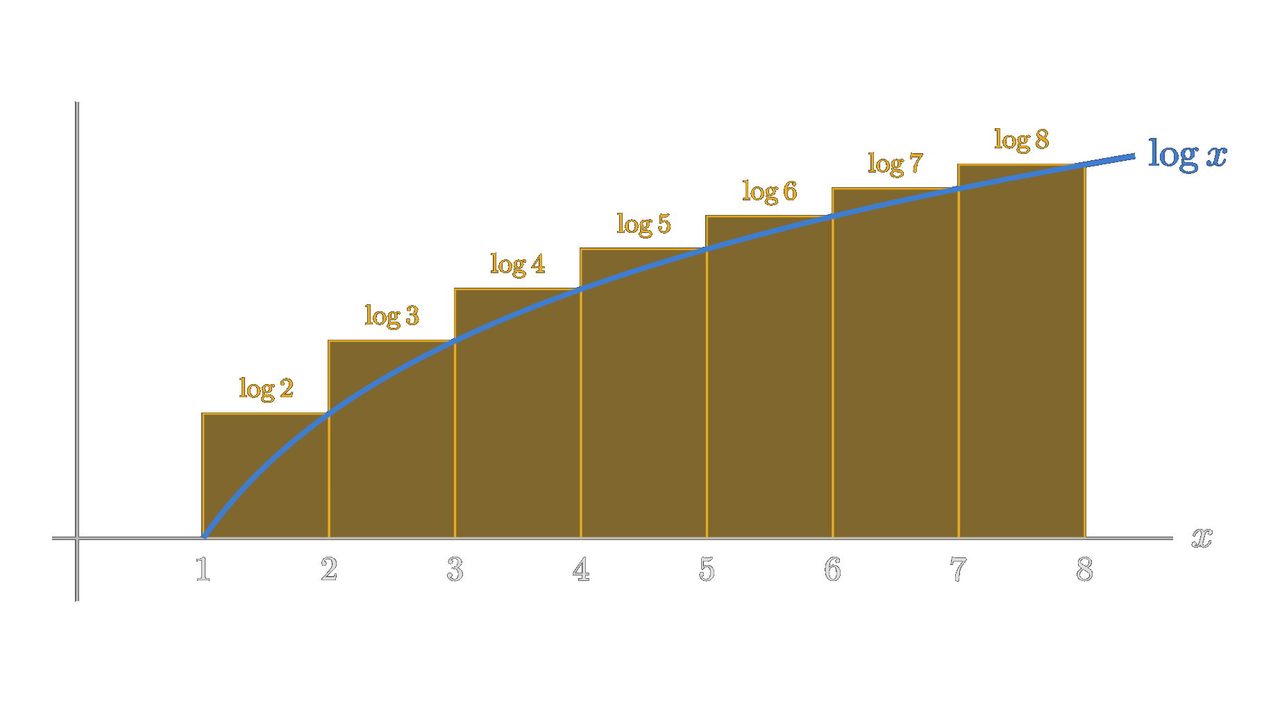
This yields
\begin{equation} \int_1^n \log(x)dx = x\log x-x \vert_1^n = n\log n - n + 1, \end{equation}which after exponentiating becomes
\begin{equation} e\frac{n^n}{e^n}. \end{equation}That is quite similar but not the same — essentially we are missing the factor of \(\sqrt{n}\) — however the integral approximation can be improved on by realizing that the sum of the logarithms can also be interpreted as the sum of trapezoids. This sum sort of telescopes to the exact same sum of the rectangles minus the left edge of the first and the right edge of the last trapezoid. Since \(\log 1 = 0\) we only have to take the latter into account. Evidently, the integral approximates the sum of trapezoids way better compared to the sum of rectangles as shown in the following figure.
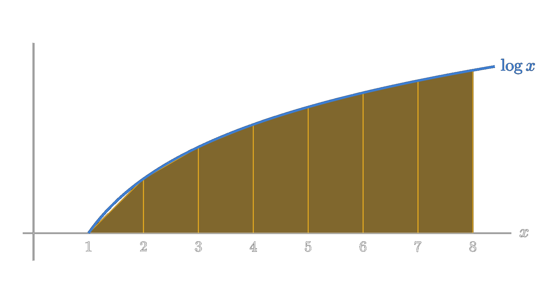
We therefore get
\begin{equation} \sum_{i=1}^n \log i - \frac{1}{2} \log n = \log n! - \frac{1}{2} \log n \approx \int_1^n \log(x)dx, \end{equation}from which we obtain
\begin{equation} e\sqrt{n}\frac{n^n}{e^n}, \end{equation}and that is essentially Stirling's approximation up to a constant factor (\(e=2.718\dots\) vs \(\sqrt{2\pi} = 2.506\dots\)).
The Middle Term
We are now going to use the result on \(\log n!\) to approximate the cumbersome factorials. Remember the main idea was to split the binomial distribution into the middle term and in an expression with which we can propagate to terms to the left and to the right of it. Using the just obtained approximation formula we get the following for the middle term, with \(n = 2m\),
\begin{equation} \begin{aligned} \log\binom{2m}{m} &= \log(2m)! - 2\log m! \\ &= \left[\left(2m+\tfrac{1}{2}\right)\log(2m) - 2m + C + \tfrac{1}{24m}\right] - 2\left[\left(m+\tfrac{1}{2}\right)\log m - m + C + \tfrac{1}{12m}\right] + \dots \\ &= 2m\log 2 + \tfrac{1}{2}\log 2 - \tfrac{1}{2}\log m - C - \tfrac{1}{8m} + \dots \end{aligned} \end{equation}The \(-2m\) and \(+2m\) cancel, the \(\log m\) terms almost cancel, and of the two constants one survives. Exponentiating and dividing by \(2^n = 2^{2m}\) (so how stands the middle term to the sum of all terms) gives, for large \(n\),
\begin{equation} M = \frac{\binom{2m}{m}}{2^{2m}} \approx \frac{\sqrt{2}}{e^{C}\sqrt{m}} = \frac{2}{B\sqrt{n}}, \qquad \log B = C = 1 - \frac{1}{12} + \frac{1}{360} - \frac{1}{1260} + \frac{1}{1680} - \dots \end{equation}And this is the result of section I of the Approximatio, where de Moivre writes the ratio of the middle term to the sum of all terms as \(\tfrac{2}{B\sqrt{n}}\), with \(B\) "the Number of which the Hyperbolic Logarithm is \(1-\tfrac{1}{12}+\tfrac{1}{360}-\tfrac{1}{1260}+\tfrac{1}{1680}\), &c."
And that is exactly the constant Stirling had figured out. But let's briefly see how he actually did it. What he essentially used is Wallis' product, something we covered already in the story Wallis' Audacious Adventure,
\begin{equation} \frac{\pi}{2} = \frac{2\cdot 2}{1\cdot 3}\cdot\frac{4\cdot 4}{3\cdot 5}\cdot\frac{6\cdot 6}{5\cdot 7}\cdots \end{equation}Look at the partial product up to the \(m\)-th factor. Pulling the factors apart, and using \(2\cdot 4\cdots 2m = 2^m m!\), it is
\begin{equation} \prod_{k=1}^{m}\frac{(2k)^2}{(2k-1)(2k+1)} = \frac{1}{2m+1}\left(\prod_{k=1}^{m}\frac{2k}{2k-1}\right)^2 = \frac{1}{2m+1}\left(\frac{(2\cdot 4\cdots 2m)^2}{(2m)!}\right)^2 = \frac{1}{2m+1}\left(\frac{2^{2m}}{\binom{2m}{m}}\right)^2. \end{equation}Wallis tells us that this tends to \(\tfrac{\pi}{2}\), and therefore
\begin{equation} \frac{\binom{2m}{m}}{2^{2m}} \approx \sqrt{\frac{2}{\pi(2m+1)}} \approx \frac{1}{\sqrt{\pi m}}. \end{equation}Compare this with de Moivre's \(\tfrac{2}{B\sqrt{n}} = \tfrac{\sqrt{2}}{B\sqrt{m}}\), and out comes \(B = \sqrt{2\pi}\). De Moivre puts it like this: his "worthy and learned Friend Mr. James Stirling" had found "that the Quantity B did denote the Square-root of the Circumference of a Circle whose Radius is Unity", so that with this circumference \(2\pi\) the middle term becomes simply
\begin{equation} M \approx \frac{2}{\sqrt{2\pi n}}. \end{equation}Something that is not necessarily needed for a numerical evaluation of the approximation of the middle term but nevertheless adds significant estatic pleasing to the result as de Moivre points out.
And with that we can also answer Mr. Cuming's question from the beginning without having to evaluate unwieldy factorial expressions:
\begin{equation} E\left|X - \tfrac{n}{2}\right| = \frac{n}{2}\,M \approx \frac{n}{2}\cdot\frac{2}{\sqrt{2\pi n}} = \sqrt{\frac{n}{2\pi}}. \end{equation}For 3600 tosses that is a deviation of about 23.9 heads on average. Notice what this says: the typical deviation grows with \(\sqrt{n}\), not with \(n\). Relative to the number of tosses it shrinks like \(\tfrac{1}{\sqrt{n}}\) — Bernoulli's law of large numbers, but now with a concrete rate attached. Keep this \(\sqrt{n}\) in mind because we will come back to it at the end of this story.
Ratio to the Middle Term
Now for the shape. We already know that the term at distance \(l\) from the middle is
\begin{equation} \frac{T_l}{M} = \prod_{i=1}^{l}\frac{m-i+1}{m+i} = \prod_{i=1}^{l}\frac{1-\frac{i-1}{m}}{1+\frac{i}{m}}, \end{equation}so in logarithmic space we are dealing with a plain sum:
\begin{equation} \log\frac{T_l}{M} = \sum_{i=1}^{l}\left[\log\left(1-\frac{i-1}{m}\right) - \log\left(1+\frac{i}{m}\right)\right]. \end{equation}Since \(i\lt m\), we can use Mercator's series once more. Expanding both logarithms up to the second order gives
\begin{equation} \begin{split} \log\left(1-\frac{i-1}{m}\right) - \log\left(1+\frac{i}{m}\right) &= -\frac{(i-1)+i}{m} - \frac{(i-1)^2 - i^2}{2m^2} + \dots \\ &= -\frac{2i-1}{m} + \frac{2i-1}{2m^2} + O\!\left(\frac{i^3}{m^3}\right). \end{split} \end{equation}We can see that both remaining terms contain the odd number \(2i - 1\) in the numerator. So, when summing over all \(i\) up to \(l\), we get the sum of the first \(l\) odd numbers \(1 + 3 + 5 + \dots + (2l-1)\), which obviously evaluates to \(l^2\). Therefore, the whole expression becomes
\begin{equation} \log\frac{T_l}{M} = -\frac{l^2}{m} + \frac{l^2}{2m^2} + O\!\left(\frac{l^4}{m^3}\right) \end{equation}For large \(n\), and hence large \(m\), we see the only term that matters is \(-\frac{l^2}{m}\). This tells us also something about at which distances \(l\) do the terms actually still matter. For \(l \ll \sqrt{m}\), the expression \(-\frac{l^2}{m}\) is almost zero, which implies that the the term \(T_l\) and the middle term \(M\) are approximately of the same size. On the other if \(l \gg \sqrt{m}\) the expression is highly negative, which means the ratio between \(T_l\) and the middle term is almost zero. This is visualized in the following image.
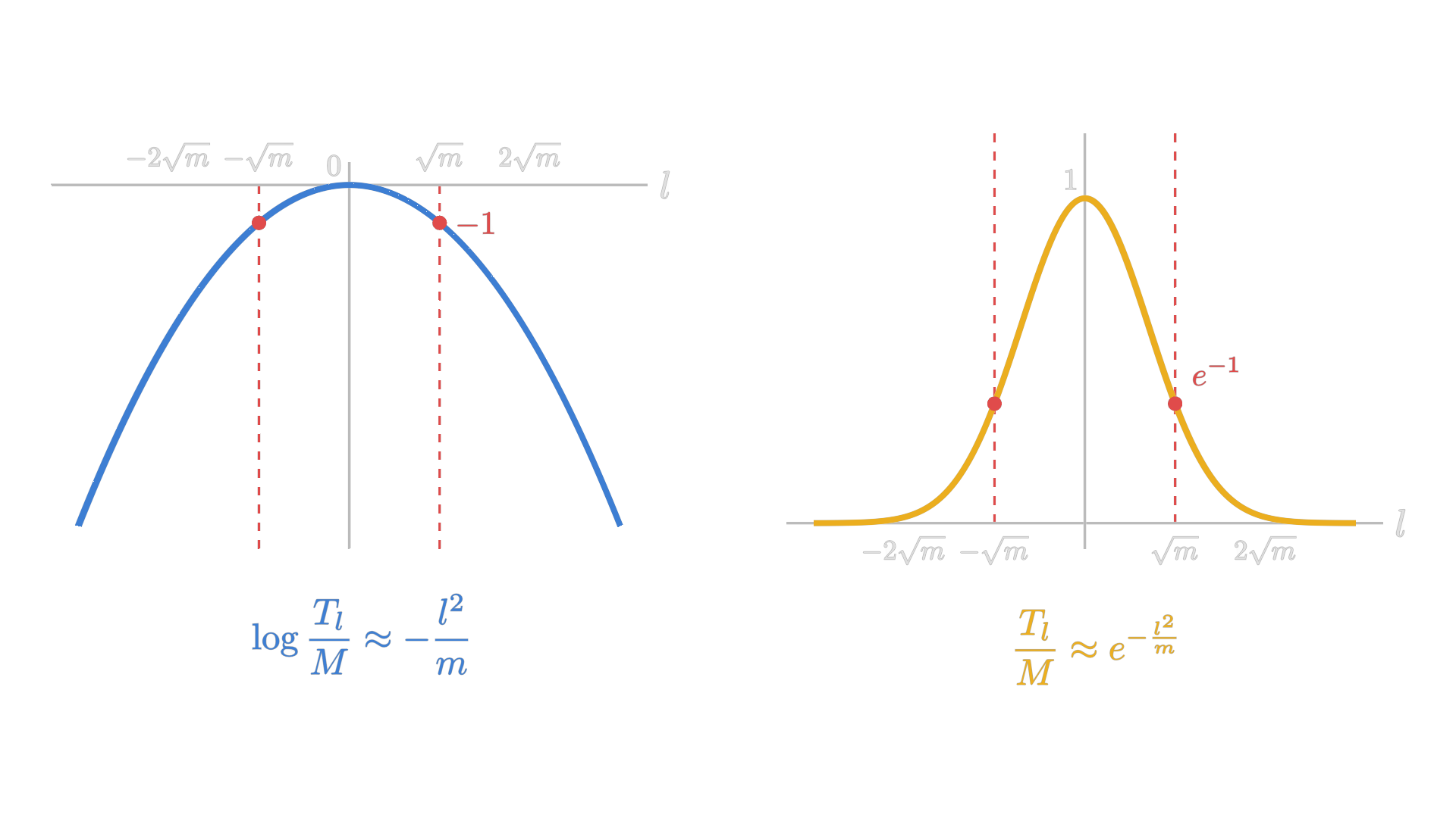
Having now figured out, what the essence of the shape is, in which the terms \(T_l\) fall off from the middle term, we can finally give an approximation formula for the binomial distribution. Because the middle term, we already now how big it is. So combining our two results and exponentiating we get
\begin{equation} T_l \approx \frac{2}{\sqrt{2\pi n}}\,e^{-\frac{2l^2}{n}}. \end{equation}And there it is. The bell curve, for the first time in history. What a significant moment in the history of mathematics.
Let's take a visual look at what we have just found out. The following image compares the exact ratios \(\tfrac{T_l}{M}\) for \(n = 50\) with the curve \(e^{-2l^2/n}\).
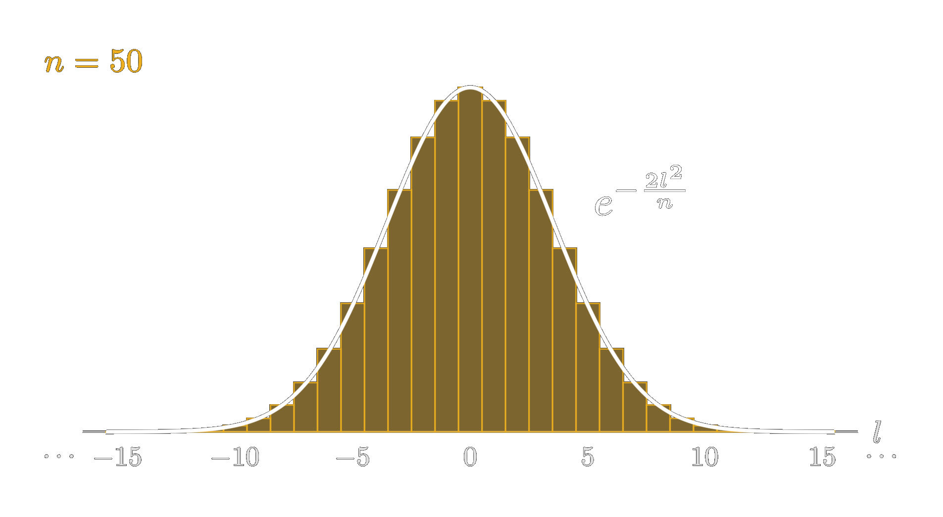
Even at this moderate \(n\) the agreement is excellent: for \(l = 5\), for example, the exact ratio is \(0.3728\), and the curve gives \(e^{-1} = 0.3679\).
Summing Multiple Terms
Let's use this approximation to go after actual probabilities. De Moivre's Lemma states the obvious: the probability that the number of heads lies between \(\tfrac{n}{2}-l\) and \(\tfrac{n}{2}+l\) is the sum of all terms in between, divided by \(2^n\). Since our \(T_j\) are already divided by \(2^n\), we simply need
\begin{equation} \sum_{j=-l}^{l} T_j \approx \sum_{j=-l}^{l} \frac{2}{\sqrt{2\pi n}}\,e^{-\frac{2j^2}{n}}. \end{equation}The terms sit at distance 1 from each other, so each of them can be seen as a strip of width 1 under the curve. For large \(n\) the curve changes only slowly from one strip to the next, and the sum can be approximated by the area under the approximation formula, that is the function of the normal curve
\begin{equation} \sum_{j=0}^{l} T_j \approx \frac{2}{\sqrt{nc}}\int_0^l e^{-\frac{2x^2}{n}}\,dx. \end{equation}But how do you evaluate this integral? There is no elementary function whose derivative is \(e^{-x^2}\). What de Moivre did have was Newton's way of dealing with such things: expand into a series and integrate term by term. The exponential series gives
\begin{equation} e^{-\frac{2x^2}{n}} = 1 - \frac{2x^2}{n} + \frac{4x^4}{2n^2} - \frac{8x^6}{6n^3} + \frac{16x^8}{24n^4} - \dots, \end{equation}and integrating every term with the good old \(\tfrac{x^{k+1}}{k+1}\) rule yields Corollary 2 of the Approximatio, the sum of the terms from the middle up to the distance \(l\):
\begin{equation} \frac{2}{\sqrt{nc}}\left(l - \frac{2l^3}{1\cdot 3\,n} + \frac{4l^5}{2\cdot 5\,n^2} - \frac{8l^7}{6\cdot 7\,n^3} + \frac{16 l^9}{24\cdot 9\,n^4} - \dots\right). \end{equation}De Moivre then takes one more elegant step: he sets \(l = s\sqrt{n}\), measuring the distance from the middle in units of \(\sqrt{n}\). Every term of the bracket then carries exactly one factor \(\sqrt{n}\), which cancels against the \(\sqrt{n}\) in the prefactor:
\begin{equation} \frac{2}{\sqrt{2\pi}}\left(s - \frac{2s^3}{3} + \frac{4s^5}{2\cdot 5} - \frac{8s^7}{6\cdot 7} + \frac{16s^9}{24\cdot 9} - \dots\right). \end{equation}The number of tosses has now disappeared. The probability of landing within \(s\sqrt{n}\) of the middle does not depend on \(n\) at all. Whether you toss 100 times or a million times, the right unit for deviations is \(\sqrt{n}\). De Moivre was well aware of how important this is — he calls \(\sqrt{n}\) "as it were the Modulus by which we are to regulate our Estimation".
This, obviously directly translates to the modern idea of the standard deviation. And it also let's you simplify this whole computation. You do not actually have to evaluate this integral up to \(l\) and then devide by whatever number of tosses \(n\) you are currently dealing with. At the end of the day you only need to know how far are you off in terms of standard deviations.
With that said let's come back to the example from the very beginning and use this approximation to evaluate the probability for it. Remeber, we had 3600 tosses, and we wanted to determine the probability that we get between 1770 and 1830 times head. Using the bare equation of the binomial distribution, we would have to evaluate extremely large factorials — an impossible task back then. However with de Moivre's approximation, it is basically a one liner. The unit, so \(\sqrt{n}\), is 60 and 1770 and 1830 lie exactly a distance of half a unit apart from the middle term. Therefore, we simply have to evaluate
\begin{equation} \frac{2}{\sqrt{2\pi}}\left(\frac{1}{2} - \frac{2}{3\cdot 2^3} +\frac{4}{2\cdot 5 \cdot 2^5} - \frac{8}{6\cdot 7 \cdot 2^7} + \frac{16}{24\cdot 9 \cdot 2^9} - \dots\right), \end{equation}which yields approximately \(0.3413\). This covers one side of the middle, from 1800 up to 1830. The other side, from 1770 up to 1800, contributes exactly the same, so the probability we are looking for is twice that, about \(0.6827\) — de Moivre himself states \(0.682688\). The exact probability, computed with todays computers, evaluates to \(0.6907\). That is fairly accurate. Therefore, I think it becomes evident how poweful this approximation was back at de Moivre's time. Because the option of brute forcing the exact solution did not exist.
For the sake of completeness, we should also mention that de Moivre extented his method for an event whose chances of happening are not equal but are given by \(p\) and \(q=1-p\) as well. In this case, he arrives at
\begin{equation} T_l \approx \frac{1}{\sqrt{2\pi npq}}\,e^{-\frac{l^2}{2npq}}. \end{equation}Conclusion
Let us step back and look at what went into this story. Mercator's series for the logarithm from 1668, and Newton's art of expanding and integrating term by term. Wallis' product for \(\pi\) from 1656, handed over by Stirling. Bernoulli's formula for the sums of powers from 1713. And a question about how much a set of coin flips deviates from the expected value, posed by Alexander Cuming. De Moivre put all of it together and what came out is an elegant way of approximating the binomial distribution for large \(n\), which on top of that turned out to be the probability density function of arguably the most important curve of probability theory, the normal distribution.
De Moivre, of course, did not see it that way — it was not possible to see it like that in his time. For him, the curve was primarily just a tool to approximate binomial sums, to avoid the cumbersome evaluation and summation of huge factorial expressions.
Why does the bell shape actually appear at all? Beside the central limit theorem — that is just the plumb general answer — we can find a more specific reason. Look at it in logarithmic space once more. The logarithm of the ratio to the middle term was a sum of many small logarithms, and what survived of their expansion was the quadratic part. In log space, the top of the hump is approximately a downward parabola — and a downward parabola in log space is precisely \(e^{-x^2}\). For the binomial, all higher-order terms die away as \(n\) grows, so the parabola is all that is left.
Of course, today we know that this is not limited to the binomial distribution. A binomial count is just a sum of independent coin tosses, and it turned out that sums of many independent random influences of almost any kind end up in the very same curve. Laplace generalized de Moivre's result in his Théorie analytique des probabilités of 1812 — which is why it is called the de Moivre–Laplace theorem today — and took the first steps towards what we now call the central limit theorem. Gauss, meanwhile, had arrived at the same curve in 1809 from a completely different direction, the theory of measurement errors. He discovered it through the lens of the general distribution for random errors and so it ended up being called Gaussian. De Moivre's priority was only brought back to wide attention in 1924, when Karl Pearson pointed to the forgotten little pamphlet of 1733.
As for de Moivre himself, he died in London in November 1754, at the age of 87. The story goes that towards the end of his life he noticed that he slept a little longer every day. Extrapolating this arithmetic progression, he computed the day on which he would sleep the full 24 hours: the 27th of November 1754. He died on that very day. Whether that is true or not — it is certainly a fitting end for a man who spent his life turning chances and randomness into something you can predict and do calculations with.