Introduction
The quadrature of the circle is one of the most prominent problems of mathematics — one that the ancient Greeks already tried to solve. Archimedes was able to show that the area of a circle equals the area of a right triangle whose base is the circumference of the circle and whose height is its radius. That transforms the problem into the question of finding an expression for the circumference of a circle — but does not solve it. There was, of course, the approximate route of fitting regular polygons with more and more sides into a circle, but that only ever yields an approximation, and it is far from anything like an exact number.
And that is essentially how far things got — for a very long time. Even about two millennia later, around the year 1600, the problem of the exact ratio between a square and a circle was still standing. Progress had been made on the numerical side: Ludolph van Ceulen pushed the polygon approximation to 35 digits (he spent most of his life on this computation, and the digits were engraved on his tombstone), and François Viète even wrote the approach out algebraically, obtaining an infinite expression of nested roots. But that was not a satisfying answer to the quadrature of the circle, and so finding what the area of a circle actually is was still an open problem.
It took until the year 1656, when a fellow named John Wallis came along. He is quite an interesting figure, as he was not a mathematician in the classical sense: he studied theology, logic and medicine, and came to mathematics remarkably late in his life — when he managed to break the latest cryptography of his time. Allegedly, at a dinner, a captured encrypted message was handed around, and Wallis solved it on that very evening in a little under two hours. That got him a position as a decipherer for the English government — and, later on, the Savilian Chair of Geometry at Oxford, with which his mathematical career actually began.
By the way, his work as a decipherer more or less marks the founding of the English secret service — another interesting story in itself, but we will stick to the mathematics today.
Anyway, only seven years after he came into contact with mathematics for essentially the first time in his life, he had already published his famous Arithmetica Infinitorum, in which he was able to solve the famous problem of determining the area of a circle — a really foundational breakthrough at that time — essentially, he discovered an infinite expression for the number \(\pi\) that is just made out of the ratio of two whole numbers. The fascinating part is how he got there — I chose the title of this story on purpose: his adventure of discovering the area of the circle had nothing to do with proving things whatsoever. It is a wild venture of spotting patterns, assuming that they hold in general, and guessing the solution — kinda like decrypting a message back in the day. He really carried his decipherer style over into mathematics.
And with that, let's take a deep dive into Wallis' Arithmetica Infinitorum and see how he did it.
The quadrature of xⁿ
The thing that differentiated the mathematics of Wallis' time the most from the mathematics of the ancient Greeks was the new algebraic perspective that included for example putting things on a concrete coordinate grid and describing shapes in terms of a function from \(x \rightarrow y\). If you look through that lens at the problem of squaring the circle you will soon find yourself dealing with the function that describes that circle, namely
\begin{equation} y = \pm\sqrt{r^2 - x^2}, \end{equation}which can be immediately derived from the core defining property of a circle — that is all points that are the same distance from a common point. For the question of the area of a circle we can simply restrict ourselves to the unit circle because we can easily generalize from there once we have a solution for that case. Also: For obvious reasons, it is sufficient if we determine the area just under the upper half-circle arc. So the function we have to deal with is essentially
\begin{equation} y = \sqrt{1 - x^2}. \end{equation}Notice that it involves a parabola, so the \(x^2\) part, and also the square root function, which is again a parabola just mirrored along the 45-degree direction. Realizing that, it seems to make a lot of sense to firstly start to pondering how one might determine the area under such curves. Also, a parabola and in general expressions of the form \(x^n\) were standard canidates for finding areas enclosed by curved lines at that time.
Therefore, Wallis initially deals with the area under such, so the parabola and the higher parabolas as he referres to them. His approach is mostly based on the ideas of Cavalieri, who had already solved those kind of questions by relying (almost) solely on geometry based arguments — something we have covered in detail in the story Cavalieri — Solving the Integral of xⁿ with Nothing but Geometry. Essentially, Cavalieri considered parallel cut lines through an area, and his reasoning rested on the fact that two collections of such lines stand in the same ratio as the areas they belong to. The one thing that differentiates Wallis' approach from Cavalieri's is that he carries this idea of parallel cut lines over into the world of arithmetic.
Take, for example, the parabola and its enclosing rectangle, and consider vertical lines through both of them. Cavalieri treated such a collection of lines as an object of its own, and the ratio between two of these objects corresponds directly to the ratio of the corresponding areas. This approach completely avoids the idea of an infinite sum — and dealing with infinity as a whole — compared to, say, the modern idea of a Riemann sum. He made it very clear that he never considered the lines as summing up to an area; he only ever talks about the ratio of two collections of lines, in the sense of the proportion theory of the ancient Greeks.
Wallis, on the other hand, while also considering these lines, determines the exact length of each of them, then explicitly computes the sum of all those lengths, and eventually puts these infinite sums into ratio. Kinda like the Riemann rectangles, only without any width — just lines. This is, of course, highly hand-wavy — because how can lines ever sum up to an area? However, for Wallis those lines were just of some infinitely small width, and he saw it in direct analog to the geometric Indivisibles from Cavalieri's work. And so, in the same manner as Cavalieri called his book Geometria indivisibilibus, so geometry of things that cannot be divided any further, he called his publication Arithmetica Infinitorum, which he himself translated as The Arithmetick of Infinites but in today's mathematical langauge it might be better translated as The Arithmetick of Infinitesimals. Still, he does not answer the question of how something infinitely small can eventually add up to some finite area.
Anyway, if we accept his approach for now and come back to our example of the parabola and its enclosing rectangle, we can easily write down those two sums. First, the vertical lines of the parabola are proportional to the square numbers. In particular, if we have \(n+1\) such lines, we get
\begin{equation} \left(\tfrac{0X}{n}\right)^2 + \left(\tfrac{1X}{n}\right)^2 + \left(\tfrac{2X}{n}\right)^2 + \dots + \left(\tfrac{nX}{n}\right)^2, \end{equation}where \(X\) is the \(x\)-coordinate up to which we consider the area under the function \(y = x^2\). Doing the same for the rectangle, which has the constant height \(X^2\), we get \(X^2 + X^2 + \dots + X^2\), see the following image.
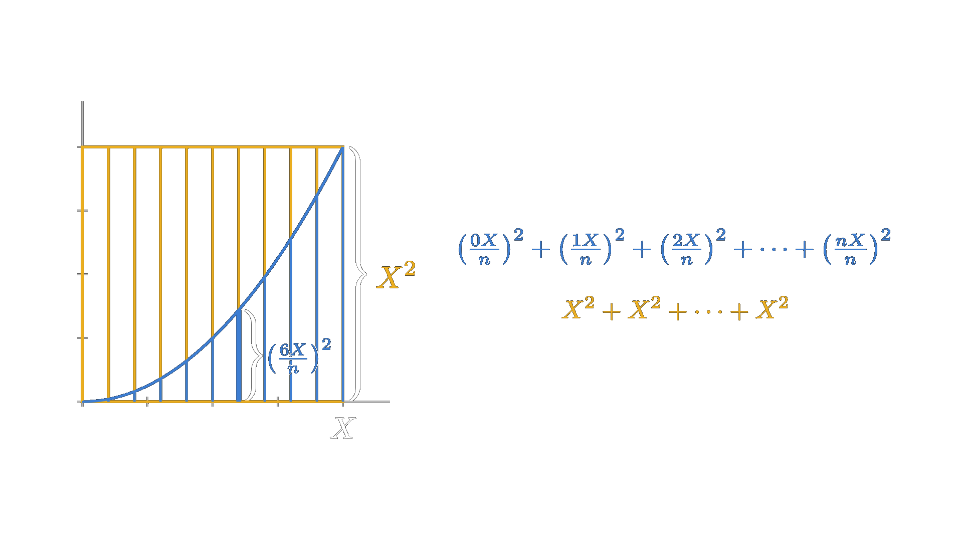
Needless to say, we can drop the common factor \(X^2\) — or, what amounts to the same, standardize things so that we consider the parabola up to \(x = 1\) — and we get for the ratio of the two sums the following expression:
\begin{equation} \frac{\left(\tfrac{0}{n}\right)^2 + \left(\tfrac{1}{n}\right)^2 + \left(\tfrac{2}{n}\right)^2 + \dots + \left(\tfrac{n}{n}\right)^2}{1^2 + 1^2 + \dots + 1^2} . \end{equation}This is not perfectly beautiful yet, but we can simply multiply the numerator as well as the denominator by \(n^2\) and get
\begin{equation} \frac{0^2 + 1^2 + 2^2 + \dots + n^2}{n^2 + n^2 + \dots + n^2} . \end{equation}In the follwing image this approach of Wallis for determining the area under a parabola is visualized.
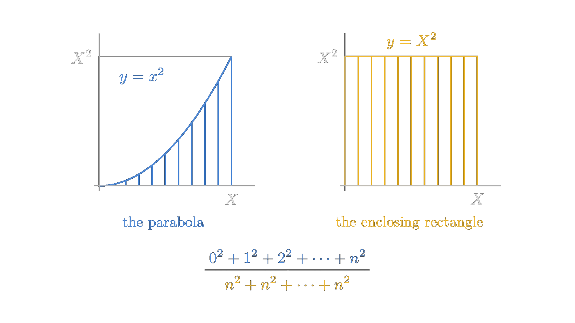
You can also get here directly, by seeing that the vertical lines of the parabola are proportional to the square numbers, and that the lines of the enclosing rectangle are then all proportional to the biggest square number. But that is just a matter of how you want to view it: either you fix what \(1\) is and express everything in fractions, or you declare your 1 such that the end of the considered area is at \(n\). Same picture — one is zooming out, the other is zooming in.
And this is by the way a good way of thinking in terms of the rational numbers. It is just the idea of: okay, what if something we labeled as one is actually made out of other somethings and each of these somethings is actually one? So the rational numbers are just natural numbers at the end of the day. This fraction notation just keeps track of how the two different perspectives of considering something as one stand to each other. Using this perspective you will see a lot of things a lot faster.
Anyway, moving on with determining the area of a parabola, Wallis then evaluates the expression for the first few \(n\)'s
\begin{equation} \frac{0 + 1}{1 + 1} = \frac{1}{2} \end{equation} \begin{equation} \frac{0 + 1 + 4}{4 + 4 + 4} = \frac{5}{12} \end{equation} \begin{equation} \frac{0 + 1 + 4 + 9}{9 + 9 + 9 + 9} = \frac{7}{18} \end{equation}and sees that it converges to \(\frac{1}{3}\). In particular, the difference to one third falls like \(\frac{1}{6}, \frac{1}{12}, \frac{1}{18}, \dots\). Hence Wallis concludes that the expression evaluates in general to
\begin{equation} \frac{0^2 + 1^2 + 2^2 + \dots + n^2}{n^2 + n^2 + \dots + n^2} = \frac{1}{3} + \frac{1}{6n}. \end{equation}Obviously, for very large \(n\) this means that the ratio between the two infinite sums will converge towards \(\frac{1}{3}\).
If we do the same for the cubic case, so \(y=x^3\), we get
\begin{equation} \frac{0 + 1}{1 + 1} = \frac{1}{2} \end{equation} \begin{equation} \frac{0 + 1 + 8}{8 + 8 + 8} = \frac{9}{24} = \frac{3}{8} \end{equation} \begin{equation} \frac{0 + 1 + 8 + 27}{27 + 27 + 27 + 27} = \frac{36}{108} = \frac{1}{3} \end{equation} \begin{equation} \frac{0 + 1 + 8 + 27 + 64}{64 + 64 + 64 + 64 + 64} = \frac{100}{320} = \frac{5}{16} \end{equation}Again, Wallis sees that the difference to one fourth behaves like \(\frac{1}{4}, \frac{1}{8}, \frac{1}{12}, \dots\) and hence he concludes that in general \(\frac{1}{4} + \frac{1}{4n}\) must hold, which in the limit yields \(\frac{1}{4}\) for the area under the curve \(y=x^3\).
Together with the obvious case for \(y=x^1\), where the result is just a simple triangle which yields \(\frac{1}{2}\) for the area, he concludes that in general we have
\begin{equation} \frac{\text{Area}(x^m)}{\text{Area}(\text{Enclosing Rectangle})} = \frac{1}{m+1}. \end{equation}Of course, without any further justification this is a highly speculative claim at this point. But for Wallis the hints were clear enough.
If you do it properly, you obviously would have to find closed formulas for the sum of the first \(n\) \(m^{th}\) powers, so in general one would have to solve
\begin{equation} \sum_{k=0}^{n} k^m \end{equation}and then compute the limit of those closed forms over \(n \cdot n^m\). So compared to Cavalieri's approach Wallis' method (if done rigorously) is not an easy shortcut because finding those closed forms was not a trivial task back in those days. We have seen in the story Stirling Numbers — The Second Kind how one would solve those kinds of sums using the approach of a difference equation. However, such methods came around the time of Stirling, and at the time of Wallis they were not known. Formulas for individual power sums did exist already (Faulhaber, for example, had published them up to the 17th power in 1631), but a general formula only came with Jacob Bernoulli in 1713 — and Wallis did not make use of any of it.
Fractional Exponents
Returning to the problem of the quadrature of the circle and realising that we can now determine the area under functions of the form \(y=x^m\) (more or less rigorously), how does that actually help us in determining the area under the function \(y=\sqrt{1-x^2}\)?
We have found a way to handle all power expressions, so if there were no square root involved in the function of a circle and the expression were, for example, simply squared instead, like
\begin{equation} y = (1-x^2)^2, \end{equation}we could just multiply things out, arrive at
\begin{equation} y = (1-x^2)^2 = 1 - 2x^2 + x^4, \end{equation}and solve each of the terms seperately and then add or subtract the resulting areas according to the sign in front of the corresponding term. So, in essence, we can now solve any polynomial expression (with integer exponents).
However, the equation for the circle is not just that, it involves a square root. But Wallis realizes that due to the fact that the square root function is exactly the inverse function of the parabola, the area under a square root function is exactly 1 minus the area under the parabola (or in general, if you do not consider the area up to \(x=1\), it will be the area of the enclosing rectangle minus the area under the corresponding parabola). This also generalizes to all the other root functions. So the area under \(y=\sqrt[n]{x}\) will be 1 minus the area under \(x^n\). In the following image this relation is visualized.
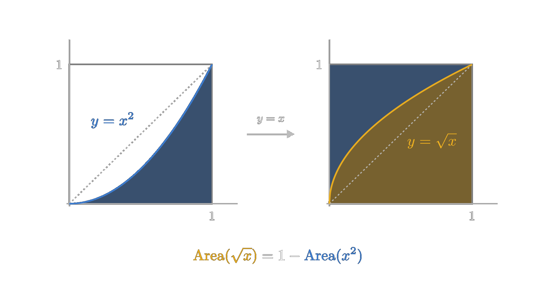
Using this insight, we can now easily extend the rule of \(\tfrac{1}{m+1}\) by considering 1 minus this expression which leads to
\begin{equation} 1 - \frac{1}{m+1} = \frac{m + 1 - 1}{m+1} = \frac{m}{m+1} = \frac{1}{1+\frac{1}{m}}. \end{equation}Looking at the result above, you will quickly realize that it is essentially the same rule, we just have to plug in \(\tfrac{1}{m}\) for the area under the \(m^{th}\) root. So in today's terms, the formula we have found for whole integer power expressions also holds for fractional power expressions. The roots just have to be considered in the exponent form, so \(\sqrt[n]{x} = x^{\frac{1}{n}}\).
But of course that was not how it worked for Wallis, because at that time the notion of a fractional exponent did not exist yet. It was he who, based on this observation, started to introduce this fractional notation for root expressions. The extension felt like the natural thing to do: when you multiply two expressions raised to the same power \(k\), the exponents add up to \(2k\); with three of them multiplied together, you get \(3k\). So if you assign the \(n\)-th root the exponent \(\tfrac{1}{n}\), then multiplying it \(n\) times will yield exactly the exponent \(1\) — the expression itself, without the root. For Wallis this again was good enough evidence that one may write
\begin{equation} \sqrt[n]{x} = x^{\tfrac{1}{n}}. \end{equation}Generalizing the problem
With that in mind, let us once again return to the function describing the circle
\begin{equation} y = (1-x^2)^{\frac{1}{2}}. \end{equation}We have now come to the point where we have solved both power expressions involved in this equation on their own. The question that remains is: can we use that to solve them here, in their combined form? Wallis does not see a concrete path to victory, even with the freshly established extension to fractional powers. However, he recognizes the core structure of the problem and generalizes on it in the hope of spotting a pattern.
For the curious minds among you who sometimes find themselves on their own mathematical adventures, that is a key take-away that we can learn from Wallis. Contrary to what is often said, that one should simplify the problem as much as possible and try to solve a smaller version of it first, it is sometimes better to generalize it even further. This makes the whole problem broader and more complex, but it might allow you to solve some cases and find some regularity in those solutions that can be extended to the case you could not solve at the beginning.
Continuing with Wallis' adventure, the generalization of the essence of the expression above is simply that we have a power expression inside (with the one-minus) and then raise the whole thing to another power. So, in a more abstract sense, we have an expression of the form
\begin{equation} y = (1-x^a)^b, \end{equation}and we want to know the area under it. Due to the symmetry of the circle, we can actually restrict ourselves to the area from zero to one.
Doing that yields another symmetry. Exchanging \(a\) and \(b\) in the sense that one is the reciprocal of the other does not change the area under this function (in this range from zero to one). Wallis takes this into account by choosing the parameters slightly differently, and he finally writes
\begin{equation} A(p, q) = \text{Area}_0^1\left(1-x^{\frac{1}{p}}\right)^q. \end{equation}We explicitly avoid the integral notation here and write out "Area" instead, because the notion of an integral did not exist in his time.
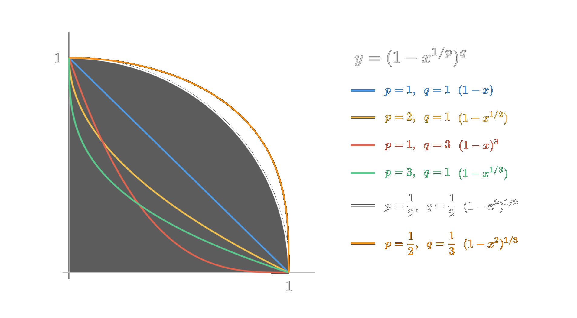
Anyway, this equation above is what Wallis tries to solve now in the hope of finding solutions for as many pairs \(p, q\) as possible — so that he can again spot some kind of pattern in them. It may then be possible to extend this pattern to the particular case of the circle that is, \(p=q=\tfrac{1}{2}\). A small selection of this generalization of our circle function is visualized in the image above.
Solving the General Case
For whole numbers \(p\) and \(q\), this is something we can actually compute with the tools from above. Take, for example, \(p = 2\) and \(q = 2\). Multiplying out the binomial gives
\begin{equation} \left(1-x^{\frac{1}{2}}\right)^2 = 1 - 2x^{\frac{1}{2}} + x, \end{equation}and now every single term is just a power of \(x\), so we can apply the \(\tfrac{1}{m+1}\) rule — including its freshly established fractional version — term by term:
\begin{equation} A(2,2) = 1 - 2\cdot\frac{1}{\frac{1}{2}+1} + \frac{1}{2} = 1 - \frac{4}{3} + \frac{1}{2} = \frac{1}{6}. \end{equation}Doing this for all small whole values of \(p\) and \(q\), Wallis notices that it is nicer to write down the reciprocals — so the ratio of the enclosing square to the area — because those turn out to be whole numbers. Arranged in a table, they look like this:
\begin{equation} \begin{array}{c|ccccc} \tfrac{1}{A(p,q)} & q=0 & q=1 & q=2 & q=3 & q=4 \\ \hline p=0 & 1 & 1 & 1 & 1 & 1 \\ p=1 & 1 & 2 & 3 & 4 & 5 \\ p=2 & 1 & 3 & 6 & 10 & 15 \\ p=3 & 1 & 4 & 10 & 20 & 35 \\ p=4 & 1 & 5 & 15 & 35 & 70 \end{array} \end{equation}And this is a familiar face: Pascal's triangle, just written into a square grid — in modern terms, the reciprocal of the area is exactly the binomial coefficient \(\binom{p+q}{p}\). Also note that the table is symmetric in \(p\) and \(q\). That is exactly the symmetry that led Wallis to put \(\tfrac{1}{p}\) into the inner exponent. If you solve \(y=(1-x^{\frac{1}{p}})^q\) for \(x\), you get \(x=(1-y^{\frac{1}{q}})^p\) — swapping \(p\) and \(q\) just swaps the roles of \(x\) and \(y\), so the graph is again only mirrored across the 45-degree direction, as visualized in the following figure.
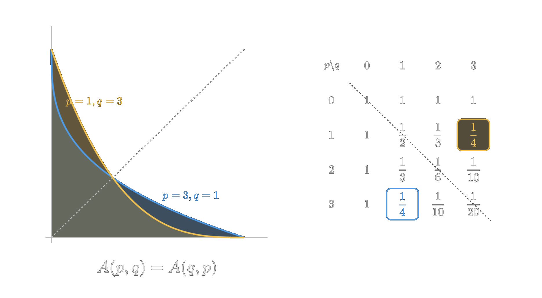
And since the curve runs from \((0,1)\) to \((1,0)\), the mirrored region is the very same region. Same area, symmetric table.
Interpolating to non-integer values
As mentioned before, the goal is now to find a pattern in these solutions when \(p\) and \(q\) are whole numbers and extent that somehow to the case of the circle, that is \(p=q=\tfrac{1}{2}.\) So, the solution we are seeking for sits right in between the rows and columns we have just evaluated. Wallis is looking for a way to interpolate to the midpoints between the rows and the columns, namely the values \(\tfrac{1}{2}, \tfrac{3}{2}, \tfrac{5}{2}, \dots\) (By the way, this is exactly where the word interpolate comes from — it was Wallis who introduced the term interpolation into mathematics, in this very book.)
We will tackle this interpolation problem in steps. First: how does one grow along a row of this table?
Let us try to spot the pattern. Looking at the whole-number entries, going from \(q-1\) to \(q\) in row \(p\) corresponds to multiplying by \(\tfrac{p+q}{q}\) — and this holds for every row. Check it, for example, in the row \(p=2\):
\begin{equation} 1 \cdot \frac{3}{1} = 3 \quad\rightarrow\quad 3 \cdot \frac{4}{2} = 6 \quad\rightarrow\quad 6 \cdot \frac{5}{3} = 10 \quad\rightarrow\quad \dots \end{equation}And here comes the decipherer again: Wallis now simply assumes that this growth rule also holds in the mid-point rows in between — so when \(p=\tfrac{1}{2}, \tfrac{3}{2}, \tfrac{5}{2}, \dots\).
He has good evidence for it. In the row \(p = \tfrac{1}{2}\), the whole-number columns can still be computed directly, because \(x^{\frac{1}{p}} = x^2\), and so \((1-x^2)^q\) is an ordinary polynomial for whole \(q\). Expanding it just like above yields the areas
\begin{equation} 1, \frac{2}{3}, \frac{8}{15}, \frac{16}{35}, \dots, \end{equation}so the reciprocals
\begin{equation} 1, \frac{3}{2}, \frac{15}{8}, \frac{35}{16}, \dots. \end{equation}And indeed, the growth rule \(\tfrac{p+q}{q}\) with \(p=\tfrac{1}{2}\) predicts the factors \(\tfrac{3}{2}, \tfrac{5}{4}, \tfrac{7}{6}, \dots\) just perfectly:
\begin{equation} 1 \cdot \frac{3}{2} = \frac{3}{2} \quad\rightarrow\quad \frac{3}{2} \cdot \frac{5}{4} = \frac{15}{8} \quad\rightarrow\quad \frac{15}{8} \cdot \frac{7}{6} = \frac{35}{16} \quad\rightarrow\quad \dots. \end{equation}Again, for Wallis this was good enough evidence, and he interpolates along the rows like that. This fills in every second column (where \(q\) is an integer) of the extended table, as shown in the following image.
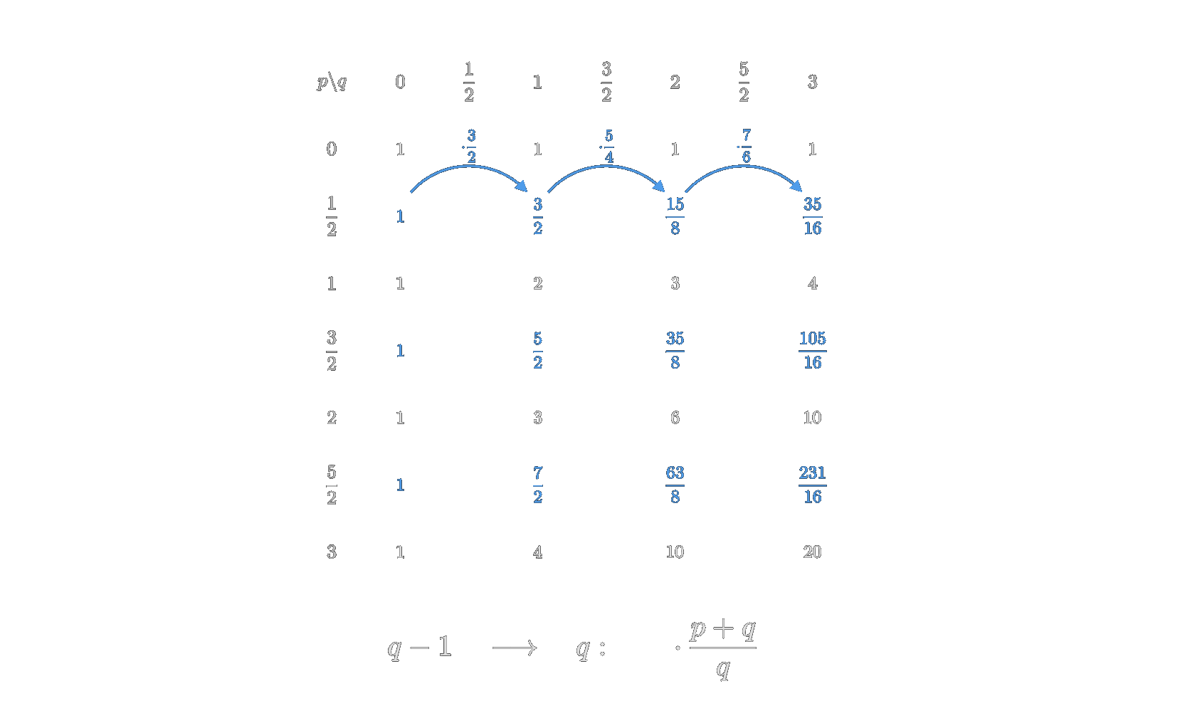
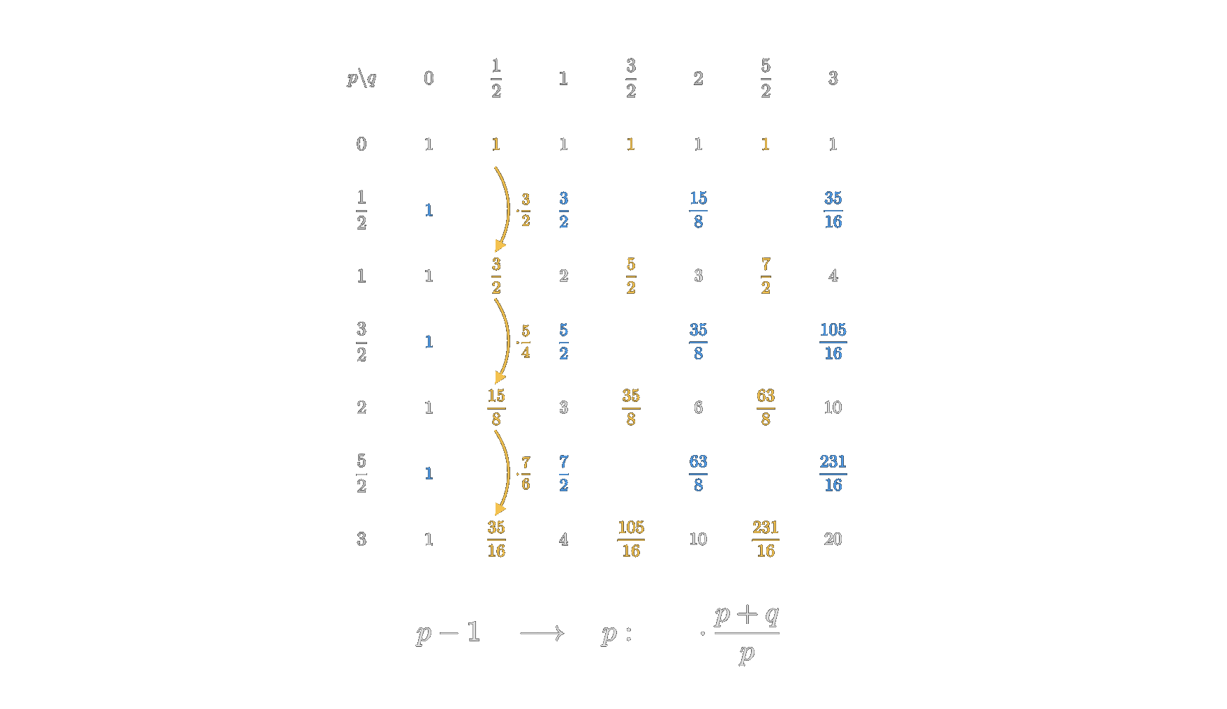
Now, as a second step, let us also check how one grows along a column of this table. The pattern is pretty similar — it is just multiplying by \(\tfrac{p+q}{p}\). Or you can take the much quicker route via the symmetry argument from before, namely switching \(p\) and \(q\). However you do it, you will see that every second row (where \(p\) is an integer) gets filled up simply by flipping the interpolated values across the diagonal. This leads to the interpolated table shown in the image below.
Now, the hard part that is still missing is of course the cells where neither \(p\) nor \(q\) is an integer. And to be frank, there is no way we can reach those — the propagation rule we assumed to hold also for non-integer values has integer step size. So if we do not start on a mixed cell (both \(p\) and \(q\) non-integer), we will never land on one.
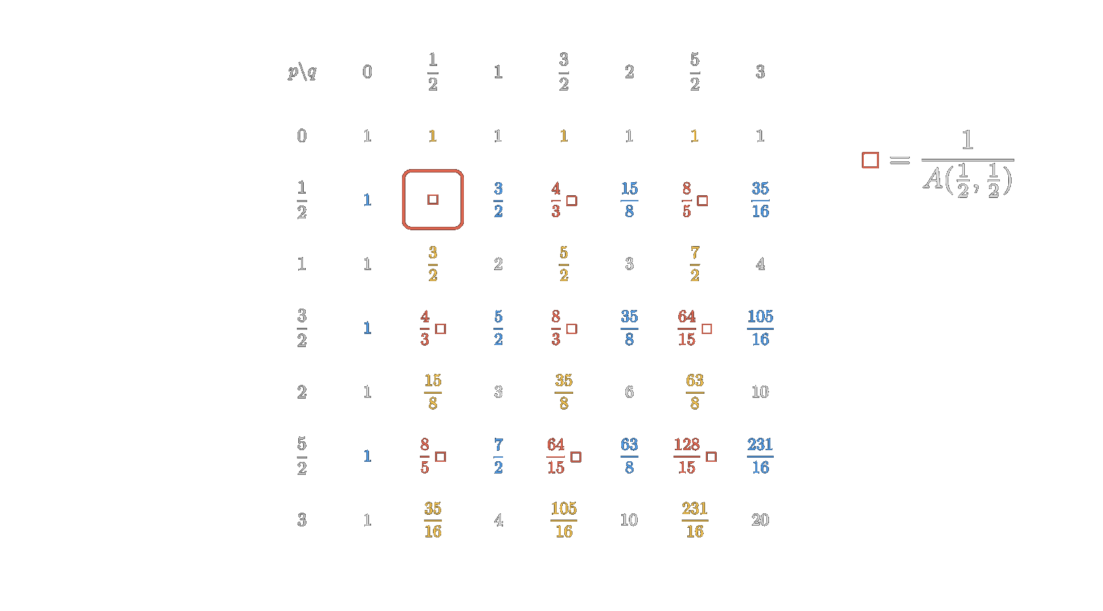
Wallis hence introduces a new symbol for the unknown value at the first grid entry of this kind, \(p=q=\tfrac{1}{2}\). The symbol he uses is a little square, \(\Box\) — and it stands for exactly the case we set out to solve. Since the table holds the reciprocals, \(\Box\) is the ratio of the enclosing square to the area of the circle — a quarter of a circle, to be precise, since we are considering the area from \(0\) to \(1\) under the function describing the upper half-circle arc.
Evidently, just giving this number a new symbol does not solve anything. But we can now again apply our rule of propagating values through the rows and columns of the table, and reach all the missing cells — as shown in the following image.
And now Wallis comes with a genius insight. Walking off along a row (or a column) sends \(q\) (or \(p\)) upward to infinity while fixing the other one — and while doing that, the area of the corresponding function keeps decreasing and decreasing, since every curve of this family lies below the previous one. Since the areas shrink as \(q\) grows, the reciprocals in our table grow, and the mixed entry at \(q=n+\frac{1}{2}\) must therefore sit between the two integer entries at \(q=n\) and \(q=n+1\). And here is the crucial part: those two integer entries differ by exactly one application of the growth factor, \(\frac{p+q}{q} = \frac{2n+3}{2n+2}\) — and that factor tends to 1 as we walk off along the row. So the two numbers enclosing our mystery entry do not merely lie close together, they close in on each other ratio-wise, as tightly as we like.
Needles to say, this also holds for the half steps, so the interpolated values. So that means in the limit, like really, really far off the start of the table, the integer values next to one grid entry of a mixed cell (\(p\) and \(q\) not an integer) will ratio-wise get arbitrarily close. At the same time, due to the assumption that the propagation rule holds also for the half steps, we can carry our mystery number from \(p=q=\tfrac{1}{2}\) over to that far off point in the table.
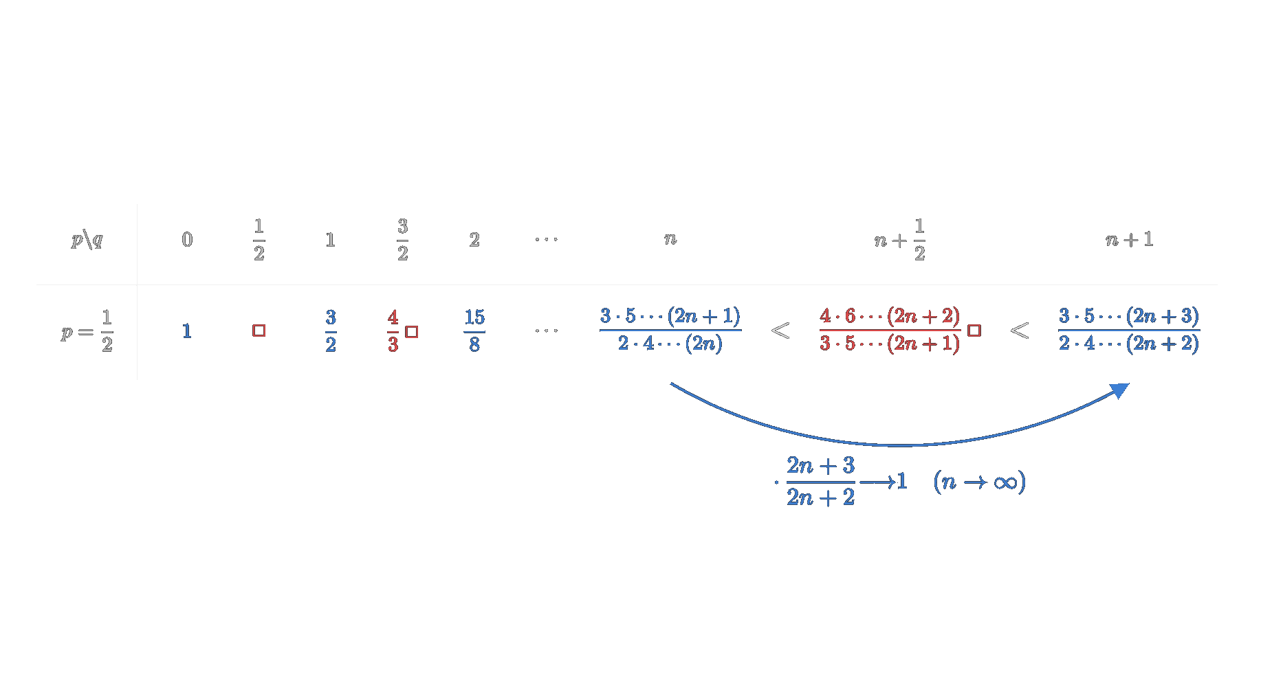
Summarizing all of that: we — or at least Wallis, depending on how thoroughly you have thought this through yourself while reading — have just found a way to sandwich (in terms of the ratio) a constant multiple of our mystery number between two numbers we know. Arbitrarily tightly.
So let us put those thoughts into equations, staying in the row of the circle, \(p=\tfrac{1}{2}\). On the one hand, we have the integer entry just before the mixed one — for very large \(q=n\), the repeated application of the growth factor \(\tfrac{p+q}{q} = \tfrac{2q+1}{2q}\) gives
\begin{equation} \frac{1}{A\left(\tfrac{1}{2},\, n\right)} = \frac{3}{2}\cdot\frac{5}{4}\cdot\frac{7}{6}\cdots\frac{2n+1}{2n}. \end{equation}Then we have the mixed entry right after it, which we express in terms of our newly introduced mystery constant by propagating \(\Box\) along the very same row — only now the growth factors are evaluated at the half-integer steps \(q = \tfrac{3}{2}, \tfrac{5}{2}, \dots\), which yields the factors \(\tfrac{4}{3}, \tfrac{6}{5}, \tfrac{8}{7}, \dots\):
\begin{equation} \frac{1}{A\left(\tfrac{1}{2},\, n+\tfrac{1}{2}\right)} = \Box\cdot\frac{4}{3}\cdot\frac{6}{5}\cdot\frac{8}{7}\cdots\frac{2n+2}{2n+1}. \end{equation}And last but not least we have the integer entry one after that mixed cell, which will evidently be given by
\begin{equation} \frac{1}{A\left(\tfrac{1}{2},\, n+1\right)} = \frac{3}{2}\cdot\frac{5}{4}\cdot\frac{7}{6}\cdots\frac{2n+1}{2n}\cdot\frac{2n+3}{2n+2}. \end{equation}Following the argument from above, we can now state that
\begin{equation} \frac{3}{2}\cdot\frac{5}{4}\cdots\frac{2n+1}{2n} \;<\; \Box\cdot\frac{4}{3}\cdot\frac{6}{5}\cdots\frac{2n+2}{2n+1} \;<\; \frac{3}{2}\cdot\frac{5}{4}\cdots\frac{2n+1}{2n}\cdot\frac{2n+3}{2n+2}. \end{equation}Now, all that is left is to rearrange for the unknown constant \(\Box\), and we have found an upper and a lower bound for the area of a quarter of a circle.
\begin{equation} \frac{3\cdot 3}{2\cdot 4}\cdot\frac{5\cdot 5}{4\cdot 6}\cdots\frac{(2n+1)(2n+1)}{2n\,(2n+2)} \;<\; \Box \;<\; \frac{3\cdot 3}{2\cdot 4}\cdot\frac{5\cdot 5}{4\cdot 6}\cdots\frac{(2n+1)(2n+1)}{2n\,(2n+2)}\cdot\frac{2n+3}{2n+2}. \end{equation}By increasing \(n\) we can make those bounds arbitrarily close — in other words, we have just found a beautiful convergent product for the area of the unit circle, that is \(\pi\).
\begin{equation} \frac{4}{\pi} = \frac{3\cdot 3\cdot 5\cdot 5\cdot 7\cdot 7\cdots}{2\cdot 4\cdot 4\cdot 6\cdot 6\cdot 8\cdots} \qquad\Longleftrightarrow\qquad \pi = 2\cdot\frac{2\cdot 2\cdot 4\cdot 4\cdot 6\cdot 6\cdots}{1\cdot 3\cdot 3\cdot 5\cdot 5\cdot 7\cdots}. \end{equation}And that's the story of Wallis' product.
What did we actually find?
Let us pause for a second and appreciate the result we have just found. The formula contains nothing but whole numbers — the odd numbers, each appearing twice, over the even numbers. No roots, no polygons, no geometry whatsoever. The most geometric quantity of all, the area of the circle, expressed purely through the ratio of two products of whole numbers. Though it is an infinite product, it is still a very clear way of expressing the area of the circle.
Now you might object: didn't Viète already write down an exact infinite expression for \(\pi\), back in 1593? He did — we mentioned it in the introduction, and it was in fact the first infinite product in the history of mathematics:
\begin{equation} \frac{2}{\pi} = \sqrt{\tfrac{1}{2}} \cdot \sqrt{\tfrac{1}{2}+\tfrac{1}{2}\sqrt{\tfrac{1}{2}}} \cdot \sqrt{\tfrac{1}{2}+\tfrac{1}{2}\sqrt{\tfrac{1}{2}+\tfrac{1}{2}\sqrt{\tfrac{1}{2}}}} \cdots \end{equation}But look at it closely. Every single factor is a nested tower of square roots — an irrational number that you can never fully write down. Viète's product is really just the old polygon scheme of Archimedes written out in algebraic terms. Wallis' factors, on the other hand, are completely decoupled from any geometric perspective. For the first time, \(\pi\) was captured by arithmetic alone. Additionally, evaluated up to some finite number of terms, Wallis' expression gives a clean ratio between two whole numbers, no nested roots or other complicated terms — and that is why this result is of such significance. Whether this truly counts as the first real answer to the ancient question of the quadrature of the circle is something everyone has to decide for themselves.
For the ancient Greeks at least, the answer would most certainly be no, because the problem of the quadrature of the circle had a very specific, strict meaning: construct, using compass and straightedge alone and in finitely many steps, a square with the same area as a given circle. Wallis' product, although the Greeks would probably have admired it greatly, does not meet those requirements, and it could not — an infinite product is, by its very nature, not a finite construction. What Wallis answered is the quantitative core of the question: what is the exact ratio between circle and square, written down by honest arithmetic?
To be fair, as a tool for actually computing digits the product is dreadful; it converges extremely slowly — Ludolph van Ceulen would have given it a mild, pitying smile.
Regarding the construction version of the problem: That stayed open for another two centuries, and it was resolved only in 1882, when Ferdinand von Lindemann proved that \(\pi\) is transcendental — it is not a root of any polynomial equation with whole-number coefficients. Compass and straightedge, however, can only ever produce lengths that are built from whole numbers by the four basic operations (+,-,\(\cdot\),÷) and square roots, and all such lengths are algebraic numbers. Hence the Greek problem is not merely unsolved — it is actually unsolvable.
What method did we actually develop?
Another question that remains to be answered is, can we use this method of interpolating from integer values out into the vast space of fractional (or even real) values in between for other sequences of numbers as well?
The answer to this question is basically yes — but with a big caveat, as we will see in the following few paragraphs.
The first thing I thought when reading about this interpolation method was: that sounds kinda nice, maybe that can be used to interpolate the factorials as well. So without further ado, let's try exactly that.
In the following image the table — or rather the single row — representing the factorials is shown.
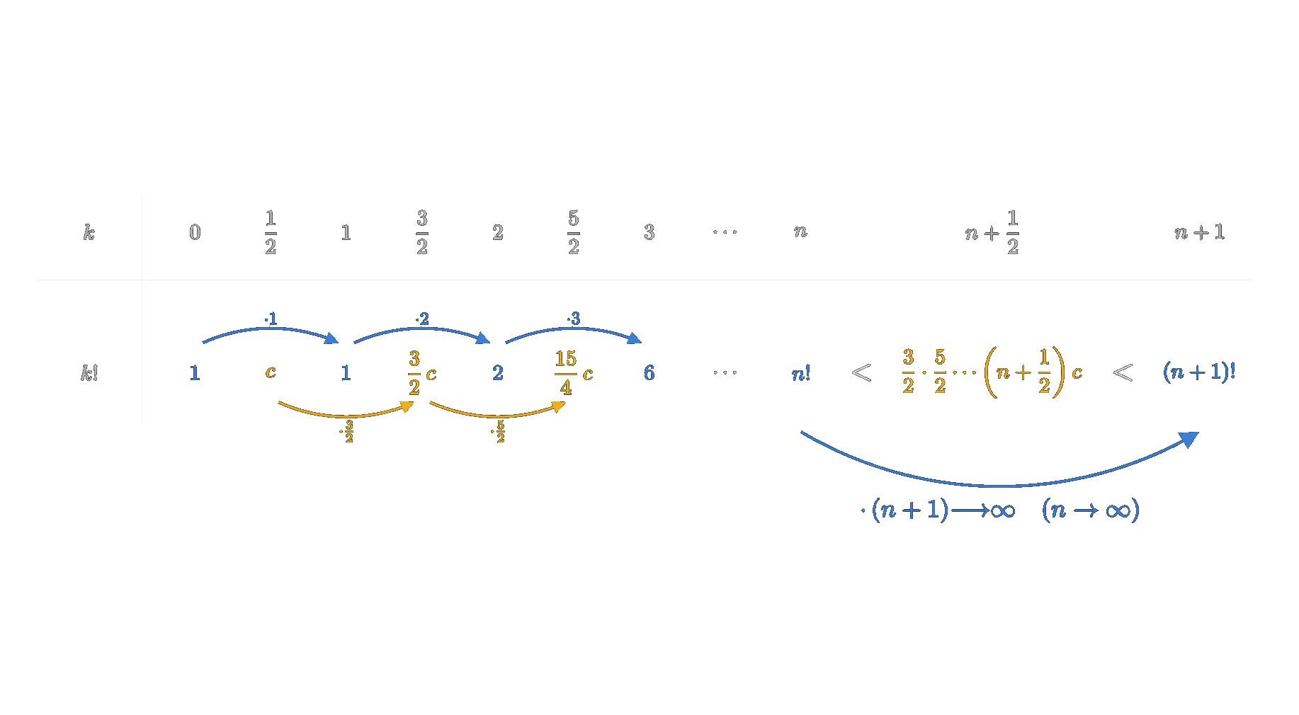
As you can see, the propagation factor for growing along this row is simply \(n\): going from \((n-1)!\) to \(n!\) means multiplying by \(n\). Again we extend the table to the midpoints \(\tfrac{1}{2}, \tfrac{3}{2}, \tfrac{5}{2}, \dots\). Similarly to before, we cannot determine the value at \(k=\tfrac{1}{2}\) directly, so we give it a name, a new constant \(c\) — but we assume that the propagation factor also holds at these midpoints of the table.
With that, we look at two consecutive integer entries for very large \(n\), and since the factorials are monotonically increasing, we can again construct an inequality and box in the midpoint value between the two integer values.
However, you probably already see why it will fail this time. The factorials are unbounded — so why would the entries for large \(n\) ever lie closer together? Take a look at the propagation factor: it is \(n\) itself. As \(n\) grows, the factor grows with it, so the ratio between one integer entry and the very next one keeps increasing. There is nothing to sandwich \(c\) with — the bounds fly apart, and the whole thing diverges. (Just for the record: the value that Wallis' method fails to pin down here does exist. Euler later showed, with quite different tools, that this \(c = \left(\tfrac{1}{2}\right)!\) equals \(\tfrac{\sqrt{\pi}}{2}\) — the circle sneaks in again.)
Let us take another example, the exponentials \(b^n\) — exactly what Wallis extended to fractional values at the very beginning, although only integer exponents had been defined up to that time. This interpolation might be the perfect tool to make that step rigorous, right?
So let's draw out the table with the propagation factor along the row for this case, as shown in the following image.
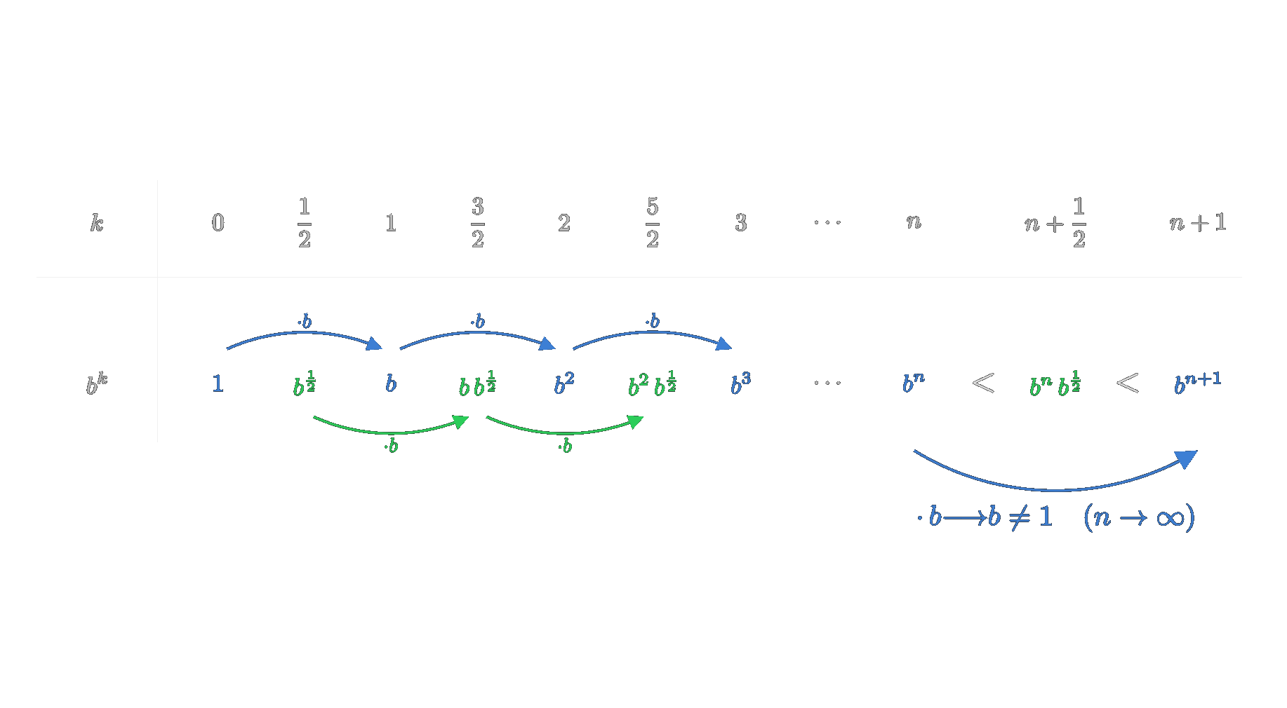
We see that the propagation factor does not depend on \(n\) at all — it is simply the constant base \(b\). That sounds like a good sign — increasing \(n\) at least does not increase the factor, right?
Well, if we construct the inequality this time and rearrange for our mystery number \(b^{\frac{1}{2}}\), we see that this constant factor is a real issue. It stays, no matter how far off we go in the table. In other words: the bounds no longer fly apart — but they never come closer to each other either. The ratio between the lower and the upper bound is stuck at \(b\).
So what we have shown using this interpolation method is merely that \(b^{n+\frac{1}{2}}\) lies somewhere between \(b^{n}\) and \(b^{n+1}\). That is not exactly something new — if it did not hold, the interpolated function would not even be monotonic, which is certainly not what we want.
The key requirement for this interpolation method to converge and produce something meaningful is that the propagation factor itself converges towards \(1\) as we walk off along the table — and this limits our possible use cases quite a bit. Essentially, we are asking for a propagation factor in which the dominant term is present in the numerator and the denominator alike. So, for example, \(\tfrac{3k^3+3}{3k^3+k}\) would be a valid case.
Nevertheless, this sandwich interpolation method is still quite remarkable, even though it is not a general answer to all interpolation problems. For those, you need to look at the sequence in logarithmic space, or at the ratios of the ratios — which eventually leads to ideas like log-convexity and, in the case of the factorials, this selects Euler's Gamma function out of all the possible interpolations. But for this story we will not blow things up further and leave it here.
Conclusion
Wallis never proved his product — not in the sense of the ancient Greeks, and not in the sense we would demand today. He computed cases, spotted patterns, assumed they persist, interpolated into unknown territory, and checked the result against everything he could check it against. His contemporaries were not exactly amused; Fermat, in particular, objected that induction of this kind is no demonstration at all. Wallis essentially shrugged: the method finds true things. And it did.
How fruitful it was became clear only a few years later. In the winter of 1664/65, a young Cambridge student worked his way through the Arithmetica Infinitorum: Isaac Newton, twenty-two years old. He picked up Wallis' interpolation idea and pushed it one decisive step further. Wallis had interpolated single numbers — the areas. Newton instead interpolated the expressions behind them: he asked what the expansion of \((1-x^2)^q\) itself looks like for \(q=\tfrac{1}{2}\), interpolating the binomial coefficients between the integer rows of Pascal's triangle. The result was the general binomial series — the binomial theorem for fractional exponents. Suddenly \(\sqrt{1-x^2}\) was an honest, if infinite, polynomial, and the area under every single term could be found with the very \(\tfrac{1}{m+1}\) rule from this story, term by term. Out of that came a series for \(\pi\) that converges incomparably faster than Wallis' product. Newton, stuck at home while the plague had shut down Cambridge (yes they had their covid years too back then), computed \(\pi\) to fifteen digits with it, and later admitted being a little embarrassed about how much time he had spent on that. Anyway, far more importantly, out of his interpolation of the coefficients came one of the pillars of calculus: expand into a power series, then integrate term by term.
So the line of inheritance runs directly through this story: Cavalieri's collections of lines, turned by Wallis into arithmetic; Wallis' pattern-guessing and interpolation, turned by Newton into the binomial series and with it another formula for the circle's area. Within about a decade, Newton and, independently, Leibniz realized that finding areas and finding slopes are inverse operations, and the laborious hunt for areas that had begun with Archimedes became a routine calculation. Euler tamed the interpolation of the factorials with the Gamma function, and the nineteenth century finally put limits and convergence on solid ground. The rigor came much later, as it usually does — the original discovery itself was made the decipherer's way.