A coin toss and its distribution
Flipping a coin - perhaps the most prominent and simplest example of probability theory in action in our universe. In this scenario, there are two outcomes: a favorable one, let's say heads, and a losing one, tails. Each outcome is equally likely, implying that both events have a probability of 50 percent.
In a more general sense, one can consider binary probabilities, where two events occur with some likelihood. Or, even better, think of one event occurring with a certain probability \(p\), and the rest of the time it simply does not occur. The latter consequently happens with a probability of \(1-p\). Such a probability distribution is one of the most fundamental, if not the most fundamental, and anyone who starts playing around with likelihoods will encounter it rather sooner than later.
This distribution is known as the Bernoulli distribution. If we call the outcome \(X\), writing the above-defined probabilities as an equation leads to
\begin{equation} P(X=k) = p^k(1-p)^{1-k}, \quad k \in \{0,1\} \end{equation}which is just a compact way of saying \(X\) being one has a probability of \(p\) and \(X\) being zero of \(1-p\). So we used 0 and 1 to indicate the two possible outcomes.
A natural question arises: what happens if we observe the outcome of a Bernoulli-distributed variable \(n\) times? For example, what if we flip a coin \(n\) times? In this case, the distribution changes - there are no longer just two possible results whose frequency is solely determined by the probability \(p\) but multiple ones. Those results represent outcomes such as the event never occurred, occurred once, twice, and so on, up to \(n\) times. Intuitively, it also seems that the outcomes at the extremes, such as getting heads only once in ten coin flips, are less likely than, say, getting heads five times. However, how can we formally express this concept? How do we derive a formula for this distribution?
N Bernoulli trials
Let's start with a specific example and consider 2 Bernoulli trials. What can happen in this setting? Well, in the first attempt, the event can either occur or not. And then the same for the second attempt. So if we list all possible outcomes, it looks like this:
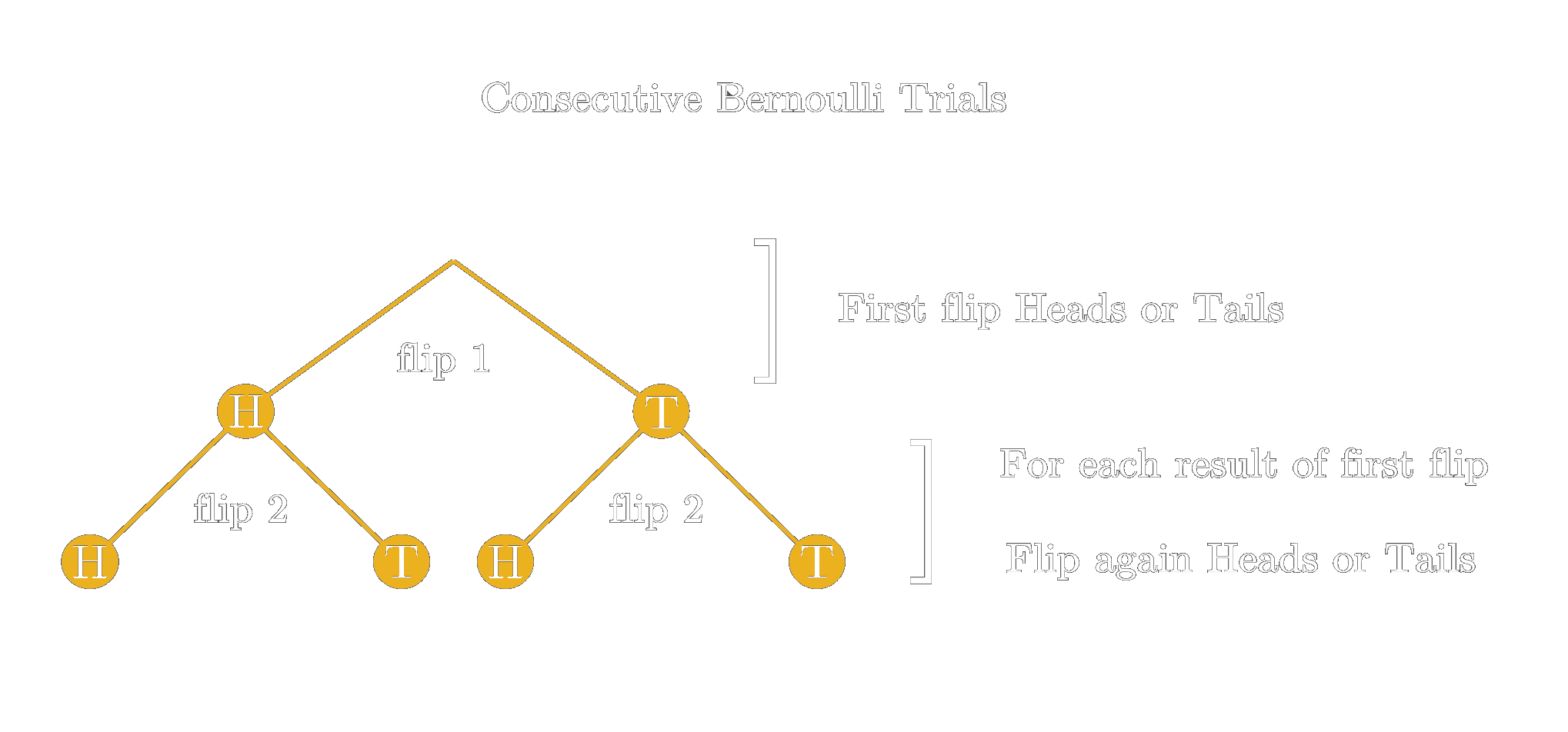
As you can see it results in a tree structure. For the first one, either heads or tails can occur (or 1 and 0 if you prefer the abstract representation). And then for each of these results, heads or tails can occur again. For further cases, such as 3 and 4 Bernoulli trials, the tree structure grows, as can be easily imagined by looking at above figure.
However, let's stick with the case of two Bernoulli trials for now. The possible outcomes increase by 1 compared to the Bernoulli distribution, since now the event (e.g. flipping heads) can occur 0, 1, or 2 times. If \(n\) is the number of trials, then the set of possible results is given by \(\{0,1,2,\dots,n\}\), which are \(n+1\) different possible results in total.
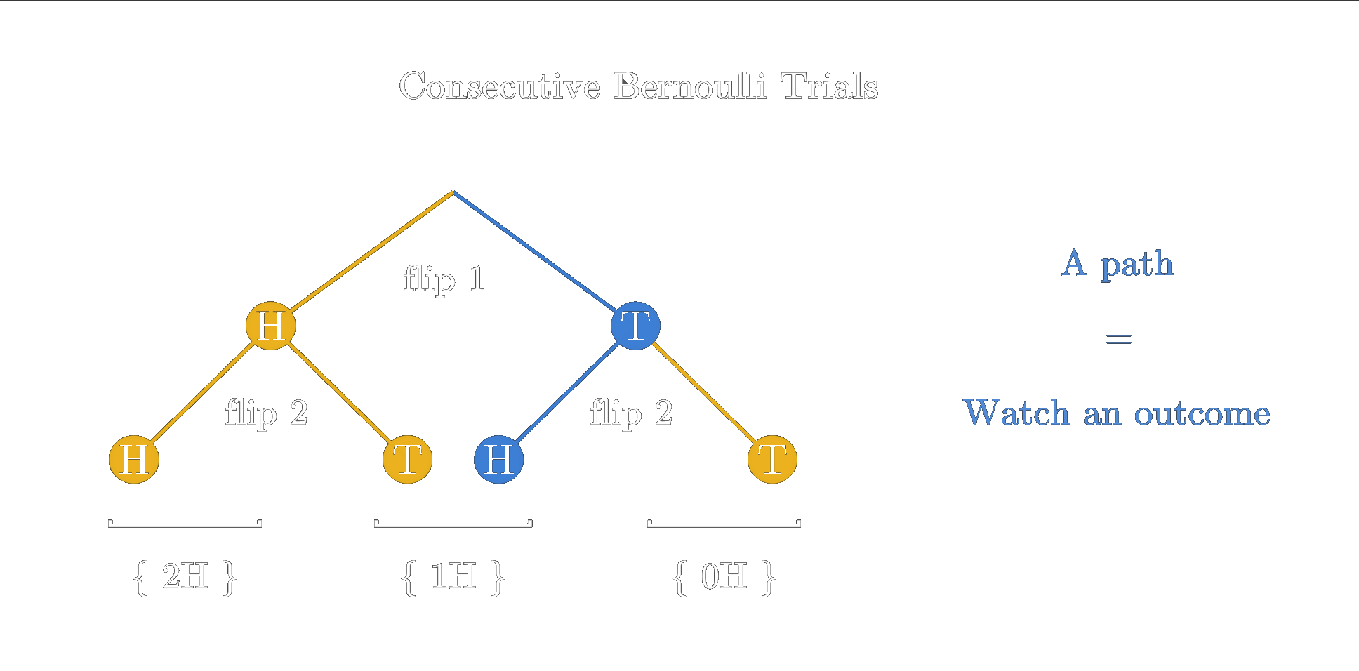
If we follow down a specific path in the tree structure, we watch a single outcome of \(n\) Bernoulli trials. We can easily compute the probability for this happening by just multiplying the probabilities. So, for example, in our 2 Bernoulli trials, the probability of the desired event happening in the first trial and not happening in the second one is evidently given by \(p(1-p)\).
But why are we actually allowed to just multiply? This works because the trials do not influence each other - a coin has no memory and does not care what it showed in the flip before. In the language of probability theory, the trials are independent. On top of that, we assume the probability \(p\) stays the same for every single trial. Both assumptions are quietly hidden in our tree, but everything that follows builds on them.
However, if we are seeking the overall probabilities for the possible results (event occurred 0, 1, or 2 times), this is far from capturing the whole picture. This is due to the obvious reason that multiple paths lead to the same result.
Therefore, in order to arrive at a final formula for the probabilities of all the possible results, we have to multiply the probability for a path leading to a specific result by the number of possible paths to that very same result. This works because all paths leading to the same result are equally likely - they contain the same number of occurrences and non-occurrences, just in a different order.
So let us step back a little and think about what we actually have to solve to be able to determine the number of possible paths to one result. If we assume we look for the result of \(k\) occurrences after \(n\) trials, then we do not know when the \(k\) occurrences happened. For example, assume we make 4 trials and we seek to find the probability of 2 positive outcomes during those trials. It could be that those two happened at the very beginning, but it also could be an alternation between events happening and not happening. So what we have to solve for is: how many ways are there (corresponds to how many paths are there) to distribute 2 'things' over 4 possible 'places'. Let us say this number evaluates to \(c\), then we could determine the overall probability of this result by \(c\cdot p^2 (1-p)^{2}\) - because the probability for one such specific path is again given by just multiplying the probabilities for the single Bernoulli events.
If we put the above expression into general terms, the equation from above generalizes to \(c\cdot p^k (1-p)^{n-k}\) - and the question we have to answer generalizes to: how many ways are there to distribute \(k\) 'things' over \(n\) 'places'?
Binomial coefficient
The solution to this problem turns out to be highly useful and significant, known as the Binomial coefficient. Let us delve into how we can obtain this solution and address our earlier question.
Examining the following illustration, we observe \(n\) 'places' (depicted in yellow) and \(k\) 'things to distribute' (shown in blue). To provide a more concrete example, one might envision \(n\) chairs and \(k\) people.
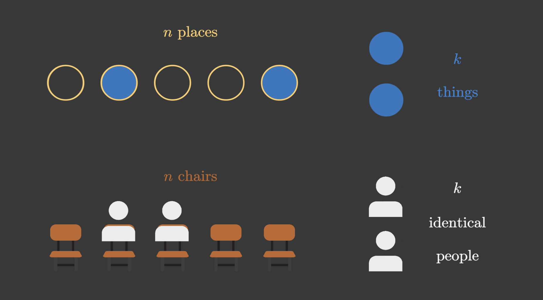
A good way of finding the number of combinations possible is to think it through person by person, or \(k\) by \(k\). The first person can choose any of the \(n\) chairs, so for him or her there are \(n\) choices. For the second person \(n-1\) choices are left, because one is always taken by the first person. So up to \(k=2\), the number of combinations is \(n (n-1)\). Needless to say, this continues for the next person, so if \(k=3\) we have \(n (n-1) (n-2)\) combinations. So in general, we could write \(n! / (n-k)!\) using the factorial sign for a compact notation. (Of course, this only works as long as there are at least as many chairs as people, so \(k \leq n\).)
However, these numbers of combinations are not quite right. Why? Because we did not take the identical person part into account. In our example of the Bernoulli trials, the event is just the event. What does this mean? This means there is no first event or second event, implying there are no \(k\) different people.
In particular, we do not care if the first person chooses the third chair and the second person the fourth chair or the first person chooses the fourth chair and the second person chooses the third chair. The persons, or in the case of the Bernoulli trials, the events are not distinguishable.
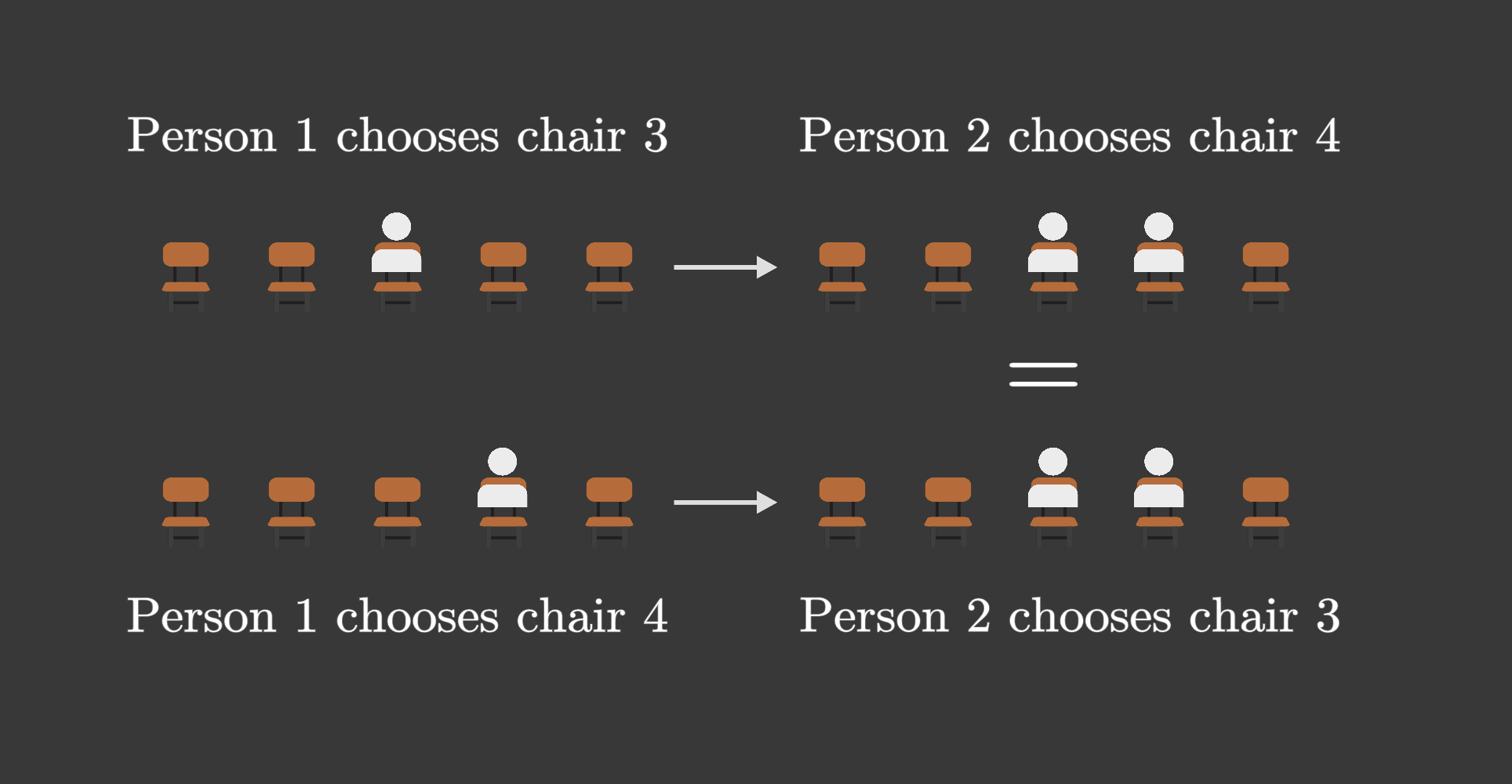
So, in fact, with our formula \(n! / (n-k)!\), we have counted a lot of combinations multiple times, which are actually the same, because we are not distributing \(k\) different events over \(n\) trials but we distribute the same event \(k\) times. However, if we knew how many times we overcounted each combination we could easily arrive at the final solution.
The question of how many times we overcounted is actually again pretty similar. We assumed \(k\) different persons, so order mattered, meaning the first person choosing the third chair and the second person choosing the fourth chair is different from the second person choosing the third chair and the first person choosing the fourth chair. However, in our case, this should be the very same combination. So the question is how many ways are there for a given set of occupied seats, to shuffle around the order by assigning a seat to a different person? Well, this is literally the same question as before, we are asking for distributing \(k\) 'things' over \(k\) 'places', however this time we are actually interested in the answer where order matters - and this we already figured out above, right? The answer is \(k(k-1)\cdots 2 \cdot 1\), which can be written compactly as \(k!\) using again the factorial notation.
So, now let us put everything together. We counted \(n! / (n-k)!\) combinations, but each of them \(k!\) times too often. Dividing by that, the question of how many ways are there to distribute \(k\) 'things' over \(n\) 'places', can be answered with
\begin{equation} {n \choose k} = \frac{n!}{(n-k)!} \frac{1}{k!}, \end{equation}
whereby the left side of the equation is a shorthand notation for the formula, usually referred to as \(n\) choose \(k\). One small detail: for \(k=0\) or \(k=n\), we run into \(0!\), which is defined to be 1. And this makes perfect sense - there is exactly one way to seat nobody, and exactly one way to fill all the chairs, and with \(0! = 1\) the formula gives us 1 in both cases.
That was kind of a long way to answer this question but hopefully, you can see why the so-derived formula makes sense. As mentioned at the beginning, this formula is actually really important and pops up all over the place in mathematics. Why? Because this question of how many ways are there to distribute \(k\) 'things' over \(n\) 'places' is just such a fundamental question to ask. Let us have a look at two other examples.
Examples of the binomial coefficient
Polynomials. Raising an expression of the form \(x+y\) to the \(n\)-th power is a quite common thing to do. What is the result of that? Well, if you write things out you will realize that everything gets multiplied with everything, so all the \(x\)'s and \(y\)'s will be multiplied, so there are again \(n+1\) different outcomes, namely \(x^n, x^{n-1}y, \dots, xy^{n-1}, y^n\). The question is again, how many times one of the terms will appear in the final result? Well, let us again look at the example of \((x+y)^n\) in the following image.
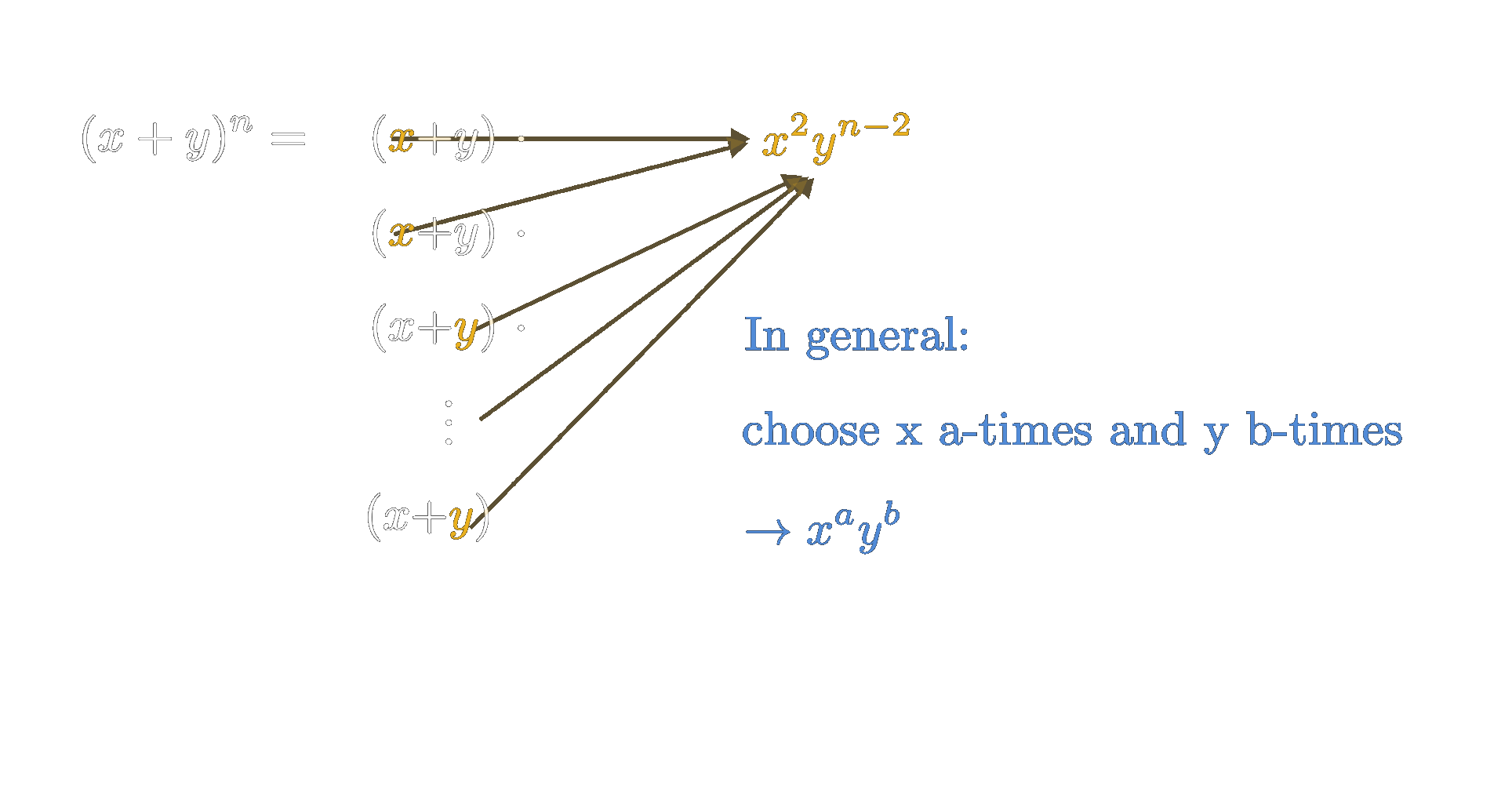
We have written the multiplication in vertical order on purpose. Notice how again, for multiplying the expression, you can choose from the first bracket \(x\) or \(y\), then for the second the same, choose again x or y, and for the third, it is again the same. Does this ring a bell in your head? That is nothing else than Bernoulli trials. This time, however, we do not take chances but aim to consider each possible combination exactly once. So when multiplying everything out, we walk down every single path of \(n\) Bernoulli trials exactly once - and as we have just seen, the number of paths leading to \(k\) times \(x\) is given by \(n! / (n-k)! / k!\).
So, for example, the term \(y^n\) will only appear once in the final result when multiplying out the expression. Why? Because there is only one path down, we always have to choose to multiply by \(y\), for all brackets. What about the term \(x^2y^{n-2}\)? Well, we have to choose \(x\) twice, all the other times, we have to multiply by \(y\). How many ways are there to do just that? Sounds like distributing 2 'things' over \(n\) 'places', so the answer is \(n! / (n-2)! / 2!\). To sum things up
\begin{equation} (x+y)^n = \sum_{k=0}^n \frac{n!}{(n-k)!k!} x^ky^{n-k}. \end{equation}
This identity is known as the binomial theorem - and it is actually where the binomial coefficient got its name from. A binomial is nothing else than a polynomial with two terms, like our \(x+y\).
Just as a little side note, what we can immediately notice here, is that we can switch \(x\) and \(y\) in \( (x+y)^n\) and it of course will result in the same expression if we multiply things out. Therefore our little formula \(n! / (n-k)! / k!\) has to have some symmetry. Evaluating the equation for \(k=0\) and \(k=n\) should lead to the same number. Likewise, for \(k=1\) and \(k=n-1\), or \(k=2\) and \(k=n-2\). Let us prove our little conjecture by evaluating the expression for \(k=i\) and \(k=n-i\):
\begin{equation} \frac{n!}{(n-i)!\,i!} = \frac{n!}{(n-(n-i))!\,(n-i)!} \end{equation}
After resolving the inner bracket, the two \(n\)'s cancel, since \(n-(n-i) = i\). So the right side is just \(n! / i! / (n-i)!\) and, noting that multiplication is commutative, we see the equality holds.
Let us move on to the second example, which will be about geometry. Essentially, it is just the geometrical interpretation of our question about how many combinations are there. Imagine a circle drawn in a two-dimensional coordinate system, centered at the origin, and now split the drawn circle by defining the same threshold value \(t\) in each coordinate. What will the resulting shapes look like?
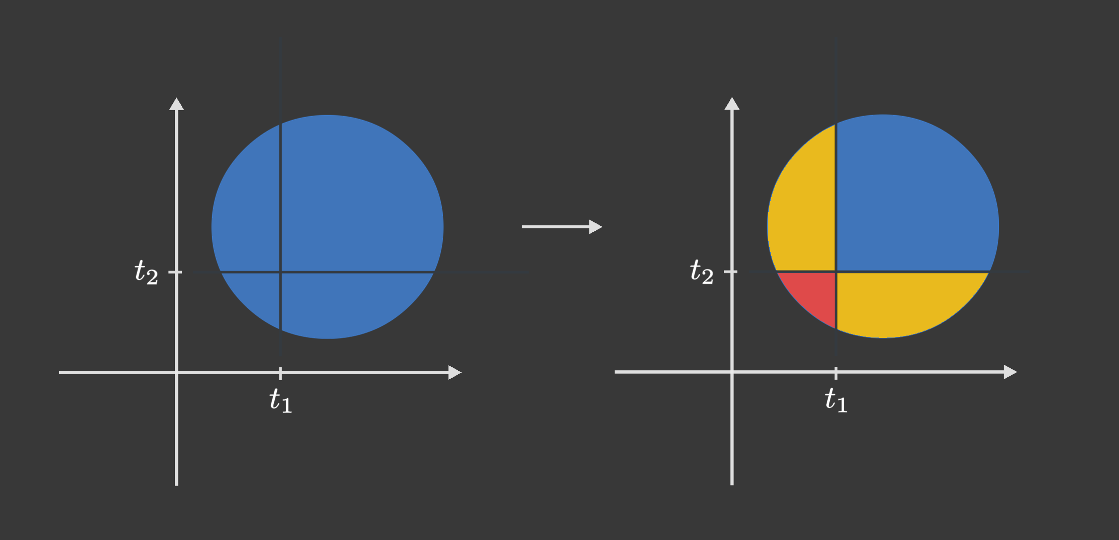
Needless to say, we are limiting ourselves hereby to the scenario where the threshold lies within the extent of the circle. And let us also assume \(t\) is not exactly zero - more on that in a moment. As you see there are 4 pieces, but 2 of them are exactly identical (just mirrored) - why is this?
That is a dumb question to ask, you might think - and maybe it is but for the sake of fun let us really rigorously reason through. We will see, everything of it has again to do with our formula \(n! / (n-k)! / k!\).
First of all, why are there four pieces? Well, that is easy. Imagine any point inside the circle, defined by two coordinates, one value per dimension. For each dimension, the value can either be greater or less than the threshold (rigorously speaking, it also can exactly equal the threshold but a single value in one dimension will never produce any area, so we can safely neglect this case). So, there are two choices that the point can make for each dimension, we could call them \(p\) and \(q\) or \(x\) and \(y\) - and since there are two dimensions, the point can make such a choice two times.
And hopefully, by now, you see where this is going. Even if we have no sense for geometry ..just being a zero-dimensional creature or whatever :) .., we could now certainly come to a conclusion about what the resulting shapes look like. And that is actually quite fascinating that this is possible.
We just showed that there are four possible ways, the first coordinate can be less or greater, and the same for the second coordinate. So all points within our circle will be in one of the four sets \(\{x_1 < t \land x_2 < t\}\), \(\{x_1 < t \land x_2 > t\}\), \(\{x_1 > t \land x_2 < t\}\) or \(\{x_1 > t \land x_2 > t\}\). What can we say about the shape of those sets? Well, that is of course heavily depending on the actual shape of the geometry we started with in the first place. But let us assume it is completely symmetrical regarding swapping the two coordinates, i.e. mirroring at the diagonal \(x_1 = x_2\) (like a circle or a square centered at the origin). Then swapping the coordinates turns every point that exceeded only the first threshold into a point that exceeded only the second one - and vice versa. So it does not matter which thresholds a point exceeded, but only how many. The shape of those sets will be solely determined by that number. And since each point can make a binary decision and can make it twice, we arrive at the very same question as for our Bernoulli trials or the polynomial expression.
Using our formula we see that for none or both thresholds exceeded, there is only one way. However, for only one threshold exceeded we see there are two ways. That means we will actually have 4 different regions after the split but only three different shapes (if the original shape is perfectly symmetrical regarding swapping the two coordinates and we use the same threshold for both).
And what about \(t=0\)? Then the cut goes right through the center and all four pieces are identical quarter circles. This does not contradict our reasoning - the circle simply has even more symmetry than the one we used. Our formula tells us which pieces are guaranteed to be identical, but there can always be some extra coincidences on top.
And there you have it. Using the binomial coefficient to reason about shapes from the perspective of a zero-dimensional creature. In the case of two dimensions this rigorous reasoning might feel like overdoing 'things' but imagine splitting a 3-dimensional sphere or a 4-dimensional cube. Then the answer is not obvious at all, however using our abstract approach with the binomial coefficient we will still be able to determine how many different shapes there are and how often each of them appears. Splitting a sphere with the same threshold in all three coordinates, for example, results in 8 pieces, which come in groups of 1, 3, 3 and 1 identical copies - so 4 different shapes. And in \(n\) dimensions, we get \(n+1\) different shapes with \({n \choose k}\) copies each, which add up to \(2^n\) pieces in total - just set \(x = y = 1\) in the binomial theorem from above and you will see why.
And that is it about the Binomial coefficient. A very important thing in mathematics that hopefully you now fully get the idea of.
Binomial Distribution
Let us come back to our original question: what does the distribution of \(n\) Bernoulli trials look like? Let \(X\) be the number of times the event occurred. We already know that every single path with \(k\) occurrences has the probability \(p^k(1-p)^{n-k}\) - and now we also know how many of those paths there are. So, putting everything together, we are now able to provide a formula for the distribution of \(n\) Bernoulli trials
\begin{equation} \begin{aligned} P(X = k) &= \frac{n!}{(n-k)!k!} p^k(1-p)^{n-k} \\ &= {n \choose k} p^k(1-p)^{n-k}. \end{aligned} \end{equation}
Let us quickly try it out with our example from above: a fair coin (\(p=0.5\)), 4 flips, and we want heads exactly twice. The binomial coefficient gives us \({4 \choose 2} = \frac{4!}{2!\,2!} = 6\) paths, and if you want, you can check this by listing them: HHTT, HTHT, HTTH, THHT, THTH and TTHH. Each of these paths has a probability of \(0.5^2 \cdot 0.5^2 = 1/16\), so overall we get \(6/16 = 0.375\).
And one more sanity check: do all the probabilities actually add up to one, as they should for any proper distribution? Here our polynomial example comes in really handy. If we set \(x = p\) and \(y = 1-p\) in the binomial theorem, we get
\begin{equation} \sum_{k=0}^n {n \choose k} p^k(1-p)^{n-k} = (p + 1 - p)^n = 1^n = 1. \end{equation}
So yes, they do - and we did not even have to calculate anything.
This distribution is known under the name Binomial Distribution. Like the Binomial Coefficient, it is extremely important in mathematics and it is one of the most fundamental discrete distributions. Once more, this stems from the fundamental query: how are the outcomes of Bernoulli trials distributed when repeated multiple times?
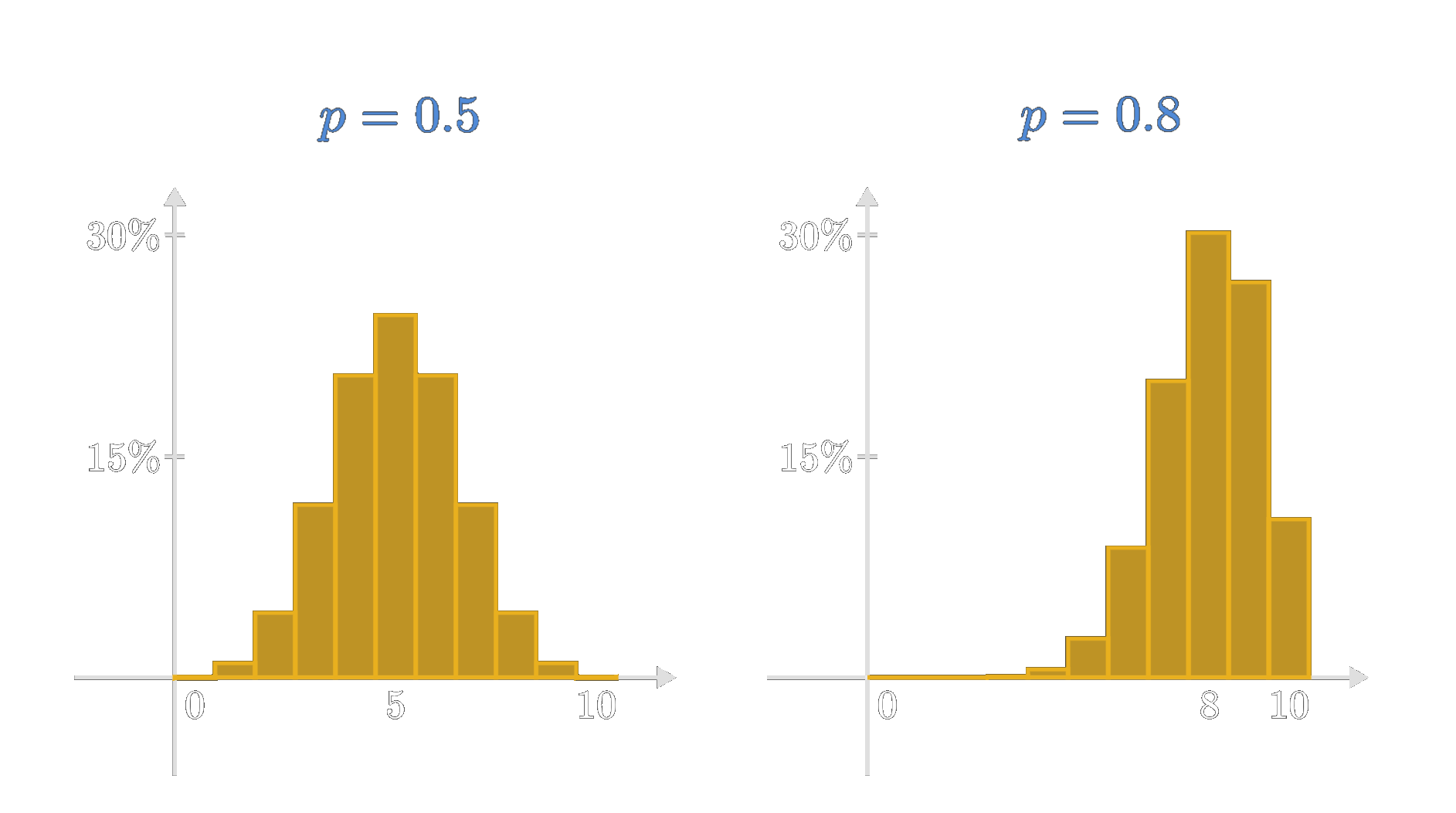
Let us have a look at what this distribution looks like. In the figure above we have evaluated the equation for two scenarios. The first one shows the case for \(p=0.5\) and the second for \(p=0.8\). In both cases, the number of trials \(n\) is 10. We see in the first scenario the distribution is perfectly symmetrical. This makes also sense on an intuitive level, since flipping heads 10 out of 10 times and flipping tails 10 out of 10 times or heads 9/10 and tails 9/10 and so on should all have the same likelihood of happening. And remember our little side note about the symmetry of the binomial coefficient? For \(p=0.5\), the factor \(p^k(1-p)^{n-k} = 0.5^n\) is the same for every \(k\), so the shape of the distribution is solely determined by the binomial coefficients - and we already proved that those are symmetrical.
In the second scenario, the distribution is no longer symmetrical but leans to the right, with its peak at \(k=8\). That is not a coincidence. If the event happens with a probability of 0.8 in each trial, then we would expect it to happen about 8 times in 10 trials. In general, this expected value is given by \(np\) - each trial contributes on average \(p\) occurrences, and we make \(n\) of them. And the peak of the distribution always sits right next to it. Outcomes far away from it, like the event happening only 2 or 3 times, become very unlikely.
Hopefully, this Story let you grasp the fundamental concept underlying the Binomial distribution. In our forthcoming Stories, we will delve into its unique properties. Specifically, we will explore the implications of increasing the number of trials. Are the outcomes more inclined to cluster around the expected value \(np\)? And does the shape of the distribution approach some limiting distribution as the number of trials approaches infinity, if we shift and rescale it appropriately? (Without that, it would simply wander off to the right and flatten out.) An equation for such a limiting distribution may prove highly beneficial, as evaluating above expression for large values of \(n\) across all possible \(k\) values can become quite laborious.
So there is still a lot left to explore. We just took our first peek into this topic. Stay tuned for exciting new Stories ahead!