Introduction
In this story, we will explore a topic in probability theory that has one of the most practical applications: statistical tests. However, instead of merely listing all the tests and accepting distributions such as the t-distribution and the chi-squared distribution as a given, we will start from the very beginning.
For example, let us consider the test of a sample variance against a theoretical variance. We will first discuss how to design the test statistic. Subsequently, we will derive a formula for the probability density function or cumulative distribution function of that test statistic. Finally, based on those findings, we will determine the probability that the sample may come from a distribution with that theoretical variance. And we are going to also think about why we did all that.
So that sounds like we have got a lot of work ahead of us and really need to take a deep dive into probability theory. But the results should be pretty exciting. This should give us a solid understanding of statistical tests, so let us dive right in.
Finding a measure for how well a variance fits
To begin our journey in developing our first statistical test, let us refer back to the example from the introduction. We have drawn a sample from a normal distribution with an unknown mean and variance. We want to determine if this normal distribution may have a certain variance \(\sigma_0^2\). Needless to say, we start by computing the sample variance of our drawn samples and look at how similar it is to \(\sigma_0^2\).
But what next? How can we determine how well this sample variance fits the theoretical one? Because obviously, they will not be 100% identical; there will in most cases be some deviation, even if \(\sigma_0^2\) is indeed the theoretical variance of the distribution we have drawn our samples from. But how much deviation is still OK?
Answering this question is actually easier than it sounds, although there will be some tricky parts along the way. All you need is a quantity, usually referred to as a test statistic, that somehow conveys information about how well the sample variance fits a theoretical one. For example, any of these quantities would meet this requirement:
- \(T = s - \sigma_0\)
- \(T = \frac{s^2}{\sigma_0^2}\)
- \(T = \frac{s^6}{\sigma_0^6}\)
- \(T = 7 \cdot \frac{s^2}{\sigma_0^2}\)
However, which one should we choose? To answer this, let us look at what we will have to do as a next step. What is the general idea of a statistical test?
A statistical test consists of a test statistic and a so-called null hypothesis, usually denoted as \(H_0\). The test statistic is a quantity that captures information about how well a certain quantity fits another, or how much a certain value deviates from a particular reference. The null hypothesis is this reference and it is the assumption we are making for determining the distribution of the test statistic. For instance, in the case of the example above, the null hypothesis would be that \(\sigma^2 = \sigma_0^2\). The case where this hypothesis is not met is the alternative hypothesis, which is usually denoted as \(H_A\).
For the test statistic, it is necessary to determine its distribution. Because then under the assumption that \(H_0\) is true, we can say how likely it is to observe a certain value for the test statistic. If the test statistic is too small or too big and hence there is little chance that we will observe it if \(H_0\) holds, we will reject the null hypothesis. Otherwise, we will say it passed the test and we cannot reject \(H_0\). For the example of our sample variance, we would say there is no evidence against our sample stemming from a normal distribution with variance \(\sigma_0^2\).
Considering the above, what can we say about the design of the test statistic in our example? We have to determine its distribution, so it will be wise to design our test statistic in a way that makes this task easy. Let us take a closer look at our candidates for the test statistic, starting with the simplest one, the ratio between the sample and the theoretical variance. When we reformulate the quantity to
\begin{equation} \frac{s^2}{\sigma_0^2} = \frac{\sum_{i=1}^n (x_i - \bar{x})^2}{(n-1)\sigma_0^2} = \frac{1}{n-1} \sum_{i=1}^n \Big(\frac{x_i - \bar{x}}{\sigma_0}\Big)^2 \end{equation}we see that this ratio actually almost standardizes our random variables \(x_i\), because we subtract the sample mean and divide by the theoretical standard deviation. The only difference is that we actually would have to subtract the theoretical mean \(\mu\) — and of course, we have to assume \(H_0\) does hold because only then \(\sigma_0\) is indeed our true variance. However, this is fine — that is the assumption for the whole test, and that is why it is called a hypothesis.
If we assumed for one second that we indeed were subtracting the theoretical mean, then our test statistic would simplify to
\begin{equation} \frac{s^2}{\sigma_0^2} = \frac{1}{n-1} \sum_{i=1}^n z_i^2, \end{equation}whereby \(z\) would be a standard normally distributed random variable. What we can also deduce is that if we had chosen
\begin{equation} \frac{(n-1)s^2}{\sigma_0^2} \end{equation}as our test quantity, so just scaling the ratio by \(n-1\), the test statistic would simplify even further to
\begin{equation} \frac{(n-1)s^2}{\sigma_0^2} = \sum_{i=1}^n z_i^2, \end{equation}again under the assumption that we had subtracted the actual theoretical mean. But what error are we actually making by only subtracting the sample mean? Let us have a look by splitting the difference from each sample \(x_i\) to the theoretical mean \(\mu\) into the difference to the sample mean \(\bar{x}\) and the difference between \(\bar{x}\) and \(\mu\). This leads to
\begin{equation} \frac{\sum_{i=1}^n((x_i-\bar{x}) + (\bar{x}-\mu))^2}{\sigma_0^2}. \end{equation}Now we can watch what happens to the \(\bar{x}-\mu\) part and see how this affects the resulting distribution.
What we essentially did is add zero. But this 'now add zero in the form of part' is utterly counterintuitive. I mean how does someone come up with that? Viewing it in the way stated above provides way more intuition and lets us understand how someone comes up with it.
After multiplying things out, the above equation can be rearranged to
\begin{equation} \sum_{i=1}^n\Big(\frac{x_i-\bar{x}}{\sigma_0}\Big)^2 + \sum_{i=1}^n\Big(\frac{\bar{x}-\mu}{\sigma_0}\Big)^2 \end{equation} \begin{equation} + 2\sum_i\frac{(x_i-\bar{x})(\bar{x}-\mu)}{\sigma_0^2} \end{equation}Notice that the last term is actually zero, due to \(\sum_i(x_i-\bar{x})\) being zero. Another perspective is that the only way of splitting up the difference \(x_i-\mu\) into two differences, such that our equation becomes just the sum of the two differences squared (without the 2ab part of the binomial expression) is to use \(\bar{x}\) as the splitting point. Remember that, because this will lead to some interesting insights, which we will discuss in another Story. For now, let us focus on the distribution of our test statistic.
Moving on, what have we found out so far? Summing things up we can state
\begin{equation} \sum_{i=1}^n z_i^2 = \frac{(n-1)s^2}{\sigma_0^2} + \sum_{i=1}^n\Big(\frac{\bar{x}-\mu}{\sigma_0}\Big)^2, \end{equation}which can be further simplified to
\begin{equation} \frac{(n-1)s^2}{\sigma_0^2} = \sum_{i=1}^n z_i^2 - n\Big(\frac{\bar{x}-\mu}{\sigma_0}\Big)^2. \end{equation}Those of you who know the distribution of the sample mean \(\bar{x}\) might see where this is going. Because as it turns out, the factor \(n\) just happens to standardize the last term as well to yet another standard normally distributed variable, which means the last term is also \(z^2\).
It turns out that we might have a shot at determining the distribution of our test statistic: all we have to figure out is what distribution a sum of squared standard normally distributed variables follows.
We waved our hands there a little bit because we also had to make sure that both terms of the subtraction, so \(\sum_{i=1}^n z_i^2\) and \(n\Big(\frac{\bar{x}-\mu}{\sigma_0}\Big)^2\) are independent because that will ensure that the subtracted term will neatly cancel with one of the \(z_i\) from the first term. However, let us not get ahead of ourselves. First, we will have to determine the distribution of the sample mean for a normally distributed variable. Secondly, it will also be advantageous to get familiar with taking a function of a random variable, because both the sample mean and the sum of squared random variables are essentially that. We have some random variables we know the distribution of, in our case \(x_i \sim \mathcal{N}(\mu,\sigma)\) and \(z_i \sim \mathcal{N}(0,1)\), and we want to know how the distribution is changing when we apply a certain function to them. In the case of the sample mean this will be a linear combination and for the other case we have this sum of squares, which is essentially the squared \(L_2\)-norm.
But before going into all those details, let us finish this Story off by seeing what we have to do after we figure out the distribution of the test statistic. That is because determining it will be quite cumbersome, and I think it definitely is worth its own Story. Let us focus on statistical tests in a more general sense here.
Applying a statistical test
First, what about the other potential candidates for our test statistic? If you choose them, you will be deviating from the standard approach, and you will find that everything does not fall into place as neatly. Determining the distribution for these alternative statistics is significantly more difficult. Therefore, we will set them aside. But of course, for a fun late-night activity, feel free to give them a try.
Assuming we have chosen our test statistic to be \(\frac{(n-1)s^2}{\sigma_0^2}\) and we determined its distribution, which we shall denote as \(\mathcal{D}\), how do we apply this statistical test now?
Let us work through this with an example. Imagine a company manufacturing steel beams that are supposed to be 3.5 meters long. The machinery involved in the production of those beams guarantees a precision of \(\sigma_0=1.5\text{mm}\), and the lengths of the beams are assumed to follow a normal distribution. To ensure the machines are working correctly, a sample of 20 steel beams is taken at the end of each day, and their lengths are measured. From these measurements, the variance is calculated. Finally, the company determines if the sample is acceptable by applying a statistical test, comparing the obtained sample variance against the theoretical precision of 1.5mm.
Based on the discussion above we choose the test statistic to be \(T = \frac{(n-1)s^2}{\sigma_0^2}\). Assuming we have solved for the distribution \(\mathcal{D}\) of \(T\) we now know how likely it will be to observe a specific value of \(T\), assuming the null hypothesis \(H_0\), that is \(\sigma^2 = \sigma_0^2\), is true.
Today the measured lengths yield a sample variance \(s^2=0.0000031\). Plugging the numbers into our test statistic leads to
\begin{equation} T = \frac{19 \cdot 0.0000031}{0.00000225} = 26.1777. \end{equation}So let us take a visual perspective on this result by looking at a plot of the probability density function \(\mathcal{D}_{PDF}\) of the test statistic \(T\).
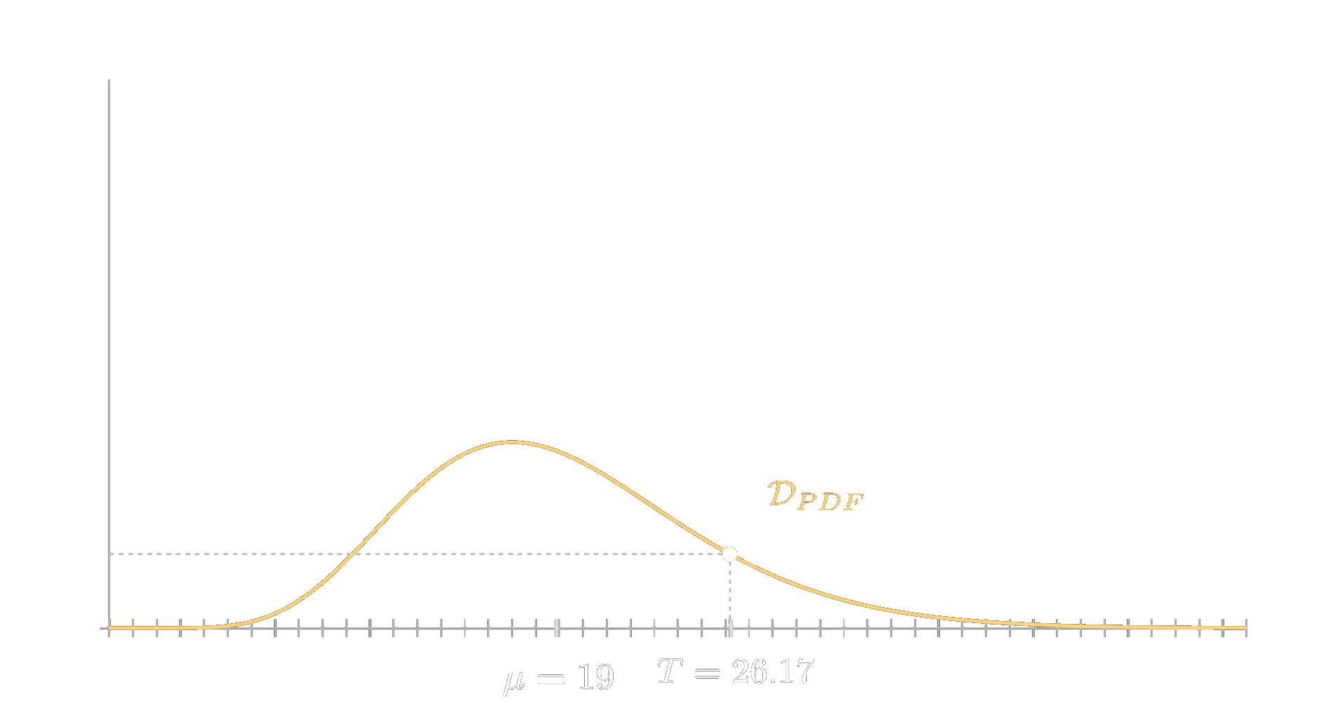
If the sample and the theoretical variance we test against were completely equal, then the ratio would be 1 and hence the value of \(T\) would be \(n-1\), so in our case 19. Deviating from this value will become increasingly unlikely as we can see in the figure above. We see that our value in this example of 26.1777 is quite a bit away and lies definitely in an area that already has a lower chance of happening if the theoretical variance were indeed \(\sigma_0=1.5\text{mm}\). However, is this already enough so that we can confidently reject \(H_0\)?
The answer to this question depends on the level of confidence we desire. Even if the test statistic is as high as 50, it is possible, albeit rare, that this could occur even if \(\sigma_0\) is indeed only 1.5 mm. Therefore, no matter how far from 19 we set our cut-off boundary for rejecting the null hypothesis, there is always a chance that we have simply observed a very rare event, and the correct move would be to not reject \(H_0\).
However, we must set this boundary somewhere; otherwise, we might as well abandon statistical tests altogether. Consequently, we accept that in some rare cases, we will make an error and reject \(H_0\) when we should not. This type of error is known as a type I error, and the probability of it occurring is denoted by \(\alpha\). The value of \(\alpha\) directly corresponds to where we set our cut-off boundary.
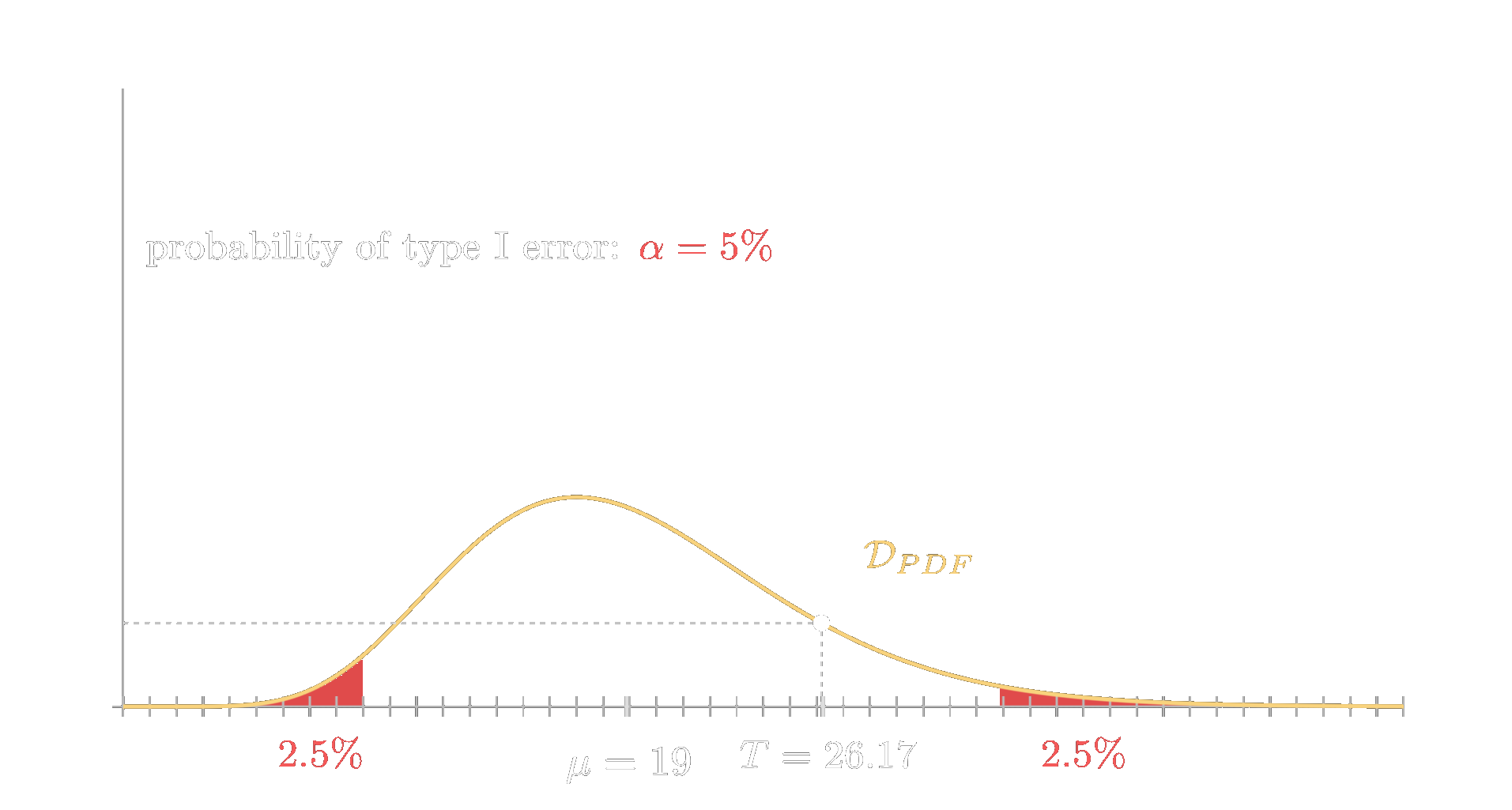
For instance, if we say we want a confidence of \(95\%\), meaning that we want to make the mistake of rejecting \(H_0\) although we should not in only \(5\%\) of cases, then this means that we set our cut-off values such that the cumulative probability at the tails of our distribution \(\mathcal{D}\) sums up to \(5\%\). So at each tail \(2.5\%\) will be outside the boundary, which are marked as red areas in the figure above.
Furthermore, there is, needless to say, also the second possible type of error, namely when we accept \(H_0\) although we should not. What is the probability of that? That depends on how far off we are by assuming \(H_0\) to be true. That is what we did in order to determine \(\mathcal{D}\). However, if \(\sigma_0\) is not the variance then our test statistic \(T\) is not fully standardized to the sum of squared standard normally distributed random variables. Hence, in this case the distribution \(\mathcal{D}\) will change. Let us find out how it changes.
Our test statistic will not be standardized by \(\sigma_0\) anymore; however, it will be by \(\sigma\). Introducing that into the equation of our test statistic we get
\begin{equation} T = \frac{(n-1)s^2}{\sigma^2} \cdot \frac{\sigma^2}{\sigma_0^2}. \end{equation}We know that the first multiplicand has the same distribution \(\mathcal{D}\), because it can be again reduced to the sum of squared standard normally distributed random variables. And the second one is just a constant. Therefore, the new distribution of \(T\), for the case where \(H_0\) is not a correct hypothesis, let us call it \(\mathcal{D}^{H_A}\), turns out to be just a horizontally stretched version of \(\mathcal{D}\), whereby the factor by which it gets stretched is \(\frac{\sigma^2}{\sigma_0^2}\). Looking at the following illustration we can see the two probability density functions (for \(H_0\) is correct and is not correct).
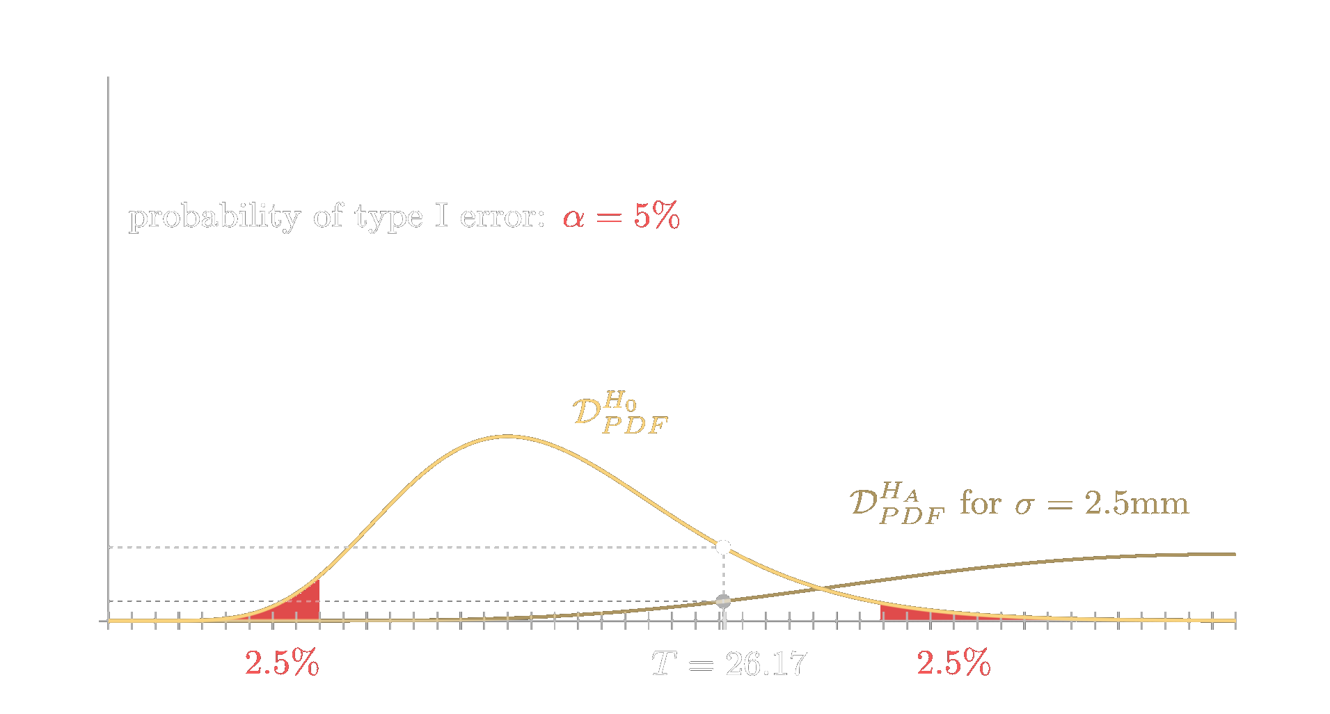
Let us elaborate on that second type of error a little more based on our example. We had \(\sigma_0=1.5\text{mm}\) but let us say it actually worsened to \(\sigma=2.5\text{mm}\) as in the figure above. So the null hypothesis \(H_0\) is not met and the alternative hypothesis \(H_A\) is true and the actual distribution of \(T\) is \(\mathcal{D}^{H_A}\), which is \(\mathcal{D}\) stretched by a factor of \(\frac{6.25}{2.25}\). However, what does this mean when we apply the statistical test?
It has the consequence that we are assuming the wrong distribution for \(T\). We are assessing the likelihoods based on \(\mathcal{D}_{PDF}^{H_0}\) and we defined a \(2.5\%\) cut-off boundary at each tail of this distribution. This means that between those values we are accepting \(H_0\). However, the test statistic \(T\) does not follow that distribution. If \(H_A\) is true it follows \(\mathcal{D}^{H_A}\). But of course, this distribution will also have some non-zero probability in our acceptance range, and in all those cases we will make an error, namely the type II error.
To determine the probability of that error, usually denoted as \(\beta\), we have to look at the actual distribution of \(T\) in that case, which is \(\mathcal{D}_{PDF}^{H_A}\). To be more precise, all we have to do is take the cumulative probability of \(\mathcal{D}_{PDF}^{H_A}\) where it falls in our acceptance range. Looking at the illustration below, we see there is quite a significant likelihood that \(T\) will take on a value in that range.
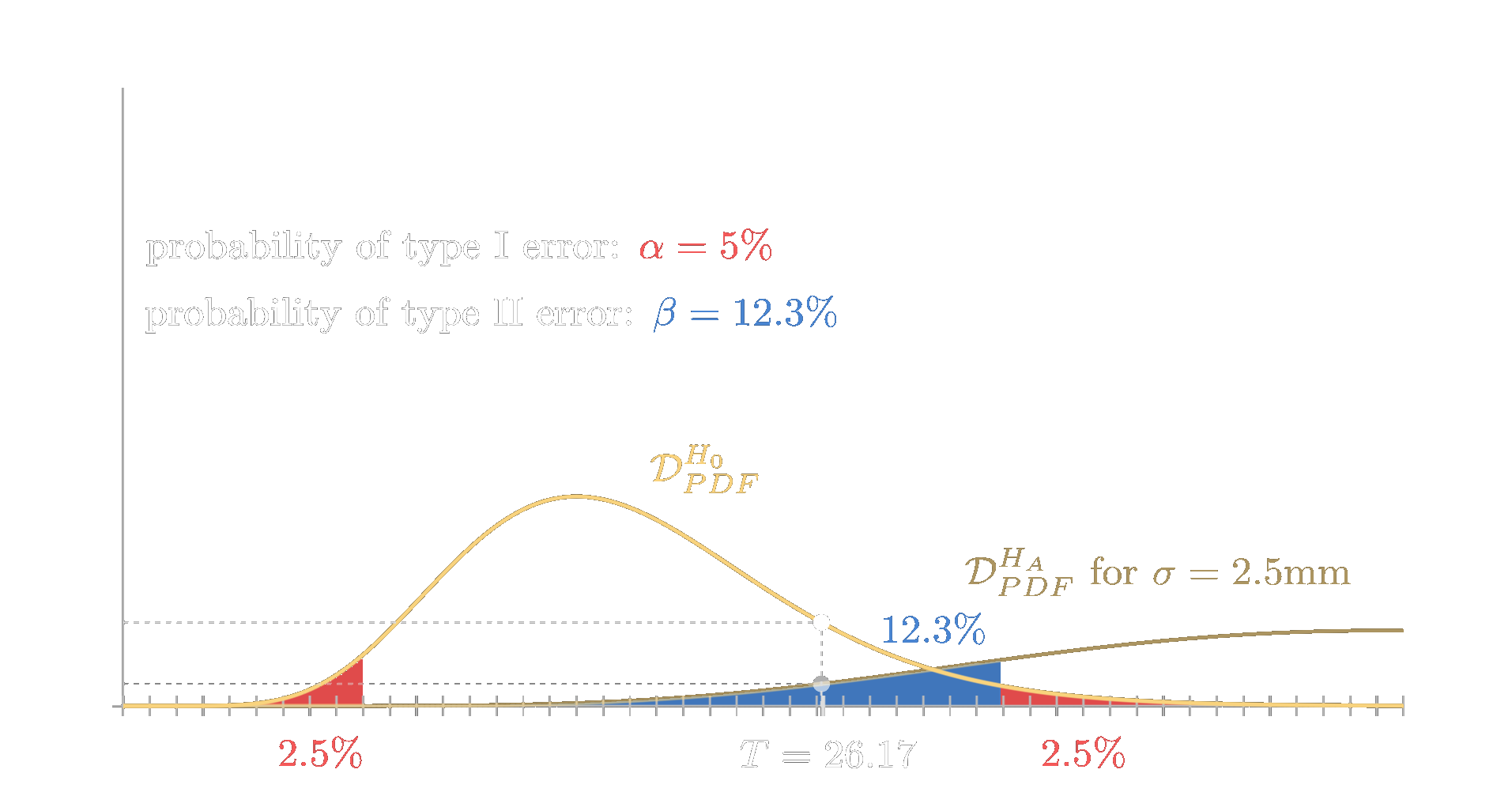
If you experiment with different values for \(\sigma\) and \(\alpha\) you will notice two things. First, increasing \(\alpha\) (which makes us more willing to accept type I errors) will generally decrease the likelihood \(\beta\) of a type II error. Second, if \(\sigma \neq \sigma_0\) (so \(H_0\) should ideally be rejected) but \(\sigma\) is actually quite close to \(\sigma_0\), the probability \(\beta\) blows up and gets tremendously high. This is because the stretched distribution \(\mathcal{D}_{PDF}^{H_A}\) is almost identical to the original distribution. Imagine if the stretched distribution was scaled down again almost matching \(\mathcal{D}_{PDF}^{H_0}\). This would cause a significant increase in the blue area, representing the probability of the type II error.
However, this is usually not a big issue. In most cases, we are not testing for exact equality. For example, if the company accepts a sample because it passed the test but the true standard deviation \(\sigma\) is actually 1.58mm instead of 1.5mm, this small difference is generally negligible. Moreover, this difference is so minor that it would be difficult to detect based on a sample alone. To identify such a small deviation, one would need to measure nearly every steel beam produced to achieve a sufficiently large sample size that would make this variation detectable.
Conclusion and outlook
With this we will wrap it up for this Story. We have delved into the foundations of statistical tests, focusing on the test of sample variance against a theoretical variance. We started by designing a test statistic, then showed why it is necessary to derive its distribution, and finally applied this to determine the likelihood of our sample coming from a distribution with the specified variance. This approach not only solidified our understanding of hypothesis testing but also provided practical insights into its application.
Moving forward, we will expand on these fundamentals by exploring other statistical tests and their applications. We will also look into more complex scenarios where multiple variables are involved and how to handle these cases efficiently. Additionally, we will work through the derivation of the different distributions of the test statistics, which we skipped a little in this Story. So stay tuned for upcoming Stories.