Introduction
To understand the derivation of the chi-squared distribution, it is important to become familiar with the concept of applying a function to a random variable, particularly to a normally distributed one. We will not go into the details of this prerequisite so if needed make sure you have read the according Stories about this topic.
Now, consider the following sum of squared independent standard normally distributed variables
\begin{equation} Y = X_1^2 + .. + X_n^2,\quad X_1,..,X_n \sim N(0,1). \end{equation}What does the distribution of this newly defined random variable look like? This might seem like an abstract question, but this sum of squared standard normal variables actually appears quite frequently in statistics.
This is essentially a problem of applying a function to a random variable, in this case, a set of multiple random variables \(X_i\) and asking what distribution the resulting variable follows. In this scenario, the problem is quite challenging, because the standard appraoch of isolationg the \(X_i\) in the above equation is not really possible. However, viewing it from a geometric perspective will ease things by a bit.
Geometric perspective on the density
When we want to determine the probability density function of a random variable, we are essentially asking how often the random variable takes on a specific value. Notice that if we set \(Y\) equal to some constant value \(y\), this defines the surface of an n-dimensional sphere, right?
\begin{equation} Y = y \Leftrightarrow X_1^2 + .. + X_n^2 = y \end{equation}Imagine the vector space where each of the \(X_i\) represents one axis. When we consider the value \(y\), it corresponds to the squared \(L_2\)-norm of the vector \((x_1,\cdots,x_n)^T\). By asking which \(x_i\) values sum to \(y\), we identify all vectors that lie on the surface of a sphere with radius \(\sqrt{y}\). This concept is illustrated in the following figure.
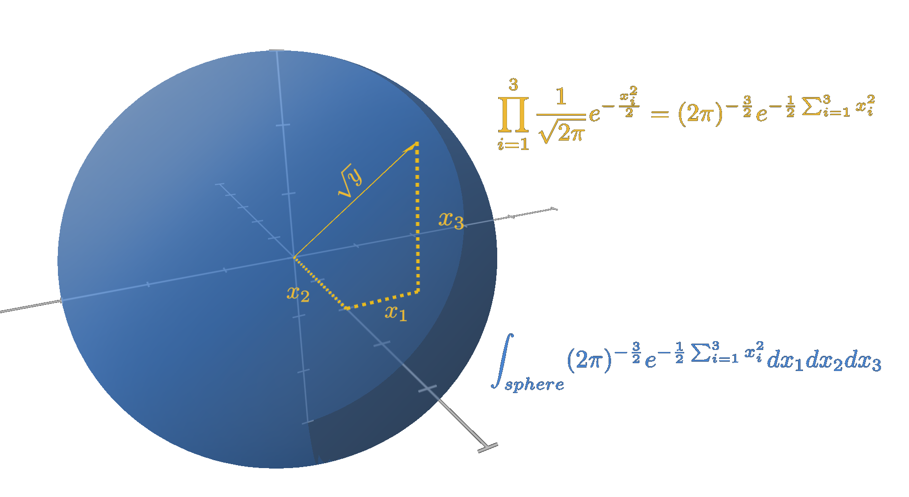
By viewing the problem from this geometric perspective, we can deduce that the probability density function of \(Y\), shortly denoted as \(Y_{PDF}\), can be represented as the integral of all probabilities within that space along the surface of a sphere with radius \(\sqrt{y}\). So let us work through that integral.
Since all \(X_i\) are independent and follow a standard normal distribution \(X_i \sim N(0,1)\) the probability of a single point in this space is given by the product of the probabilities of the individual coordinates \(X_i\). Therefore we get
\begin{equation} P(x_1,..,x_n) = \prod_{i=1}^n\frac{1}{\sqrt{2\pi}}e^{-\frac{x_i^2}{2}} = (2\pi)^{-\frac{n}{2}}e^{-\frac{1}{2}\sum_{i=1}^n x_i^2} \end{equation}Thus the probability density function at a point \(y\) can be expressed as
\begin{equation} Y_{PDF}(y) = \int_{surface}(2\pi)^{-\frac{n}{2}}e^{-\frac{1}{2}\sum_{i=1}^n x_i^2}dx_i..dx_n \end{equation}The key advantage of this geometric perspective is that we can factor out the term \(\sum_{i=1}^n x_i^2\) because, by definition, it remains constant with respect to the integral. This leaves us with the function 1 integrated over the surface of an \(n\)-dimensional sphere, which is simply the surface area. Therefore, finding the \(PDF\) of \(Y\) reduces to finding an expression for the surface area of an \(n\)-dimensional sphere, denoted \(S_{n-1}\) (We use the notation \(S_{n-1}\) because the surface is always a 'volume' of one dimension less than the dimension \(n\) of the sphere).
Concluding our geometrical insight we can state the following
\begin{equation} Y_{PDF}(y) = (2\pi)^{-n/2}e^{-\frac{y}{2}} \int_{surface}dx_i..dx_n \end{equation} \begin{equation} = (2\pi)^{-\frac{n}{2}}e^{-\frac{y}{2}} S_{n-1}. \end{equation}To be more precise, when we express the integral in terms of differentials, it reduces to the surface area multiplied by the infinitesimal thickness \(dr\). Since our probability density function is a function of \(y\), we of course need to apply the change of variables \(\sqrt{y}=r\). In terms of the locally valid linear map (i.e., differential), this implies \(S_{n-1}dr\) becomes \(S_{n-1}\frac{dy}{2\sqrt{y}}\) which means
\begin{equation} Y_{PDF}(y)dy = (2\pi)^{-\frac{n}{2}}e^{-\frac{y}{2}} S_{n-1} \frac{dy}{2y^{\frac{1}{2}}}. \end{equation}Another approach would be to consider cumulative probabilities, that is \(P(Y\leq y)\). If you examine the previous equations, you will quickly realize that this involves integrating over the entire space inside the sphere. However, when looking at the concrete equation
\begin{equation} \int_{x_i^2+..+x_n^2\leq\sqrt{y}}\prod_{i=1}^{n}\frac{1}{\sqrt{2\pi}}e^{-\frac{x_i^2}{2}}dx_1,..,dx_n \end{equation} \begin{equation} = \frac{1}{(2\pi)^{\frac{n}{2}}}\int_{x_i^2+..+x_n^2\leq\sqrt{y}} e^{-\frac{1}{2}\sum x_i^2}dx_1,..,dx_n. \end{equation}we see that we can not move the term \(e^{-\frac{1}{2}\sum x_i^2}\) out of the integral, because unlike in the direct approach to the probability density function, this expression is not constant with respect to the integral. So we will leave this approach aside for now. However, there is also a possible way to solve it via cumulative probabilities. We will come back to it at the end of this Story.
Prerequisites for the surface area of an \(n\)-dimensional sphere
Before we start on deriving an expression for the surface area, we will try to simplify the problem as much as possible. This is always a useful approach for tackling complex riddles. By breaking it down to its most simple version we only have to solve its core question. From there, we can build upon our solution by exploring how it relates to more complex variations of the problem.
In our case, it is surely advantageous to focus on a unit sphere in the familiar 2- or 3-dimensional space first. Once we have solved for that, we can examine how the surface area scales with the radius and the dimension \(n\). It could be that it is easier to determine the volume rather than the surface area. If we understand the relationship between volume and surface area, solving just for the volume alone will be sufficient as well.
Let us start with the most easy prerequisite. Let us limit ourselves to a unit sphere and try to find how it scales if we move to a different value for the radius \(r\). Since changing the radius \(r\) can be interpreted as just scaling all coordinate axes by some factor, that is a simple change of units, any \(n\)-dimensional volume will of course change by that factor to the power of \(n\). For the volume of a sphere, this means
\begin{equation} V_n(r) = r^nV_n(1). \end{equation}For the surface area, the approach is quite similar. However, since the surface area is a measure of a dimension lower than the actual volume (for a 2-dimensional sphere, the surface is a 1-dimensional line; for a 3-dimensional sphere, the surface is a 2-dimensional area), the scaling factor is \(r^{n-1}\). Consequently, we arrive at the following relationship
\begin{equation} S_{n-1}(r) = r^{n-1}S_n(1). \end{equation}Having established how the volume and the surface scale with the radius \(r\), the next step will be to find the direct relationship between the surface and the volume. For that, we will take a geometric perspective again. Imagine a sphere approximated by thin cones, with their tops lying in the center of the sphere. In the limit, if the size of these cones gets towards zero and the number of cones increases towards infinity, the sum of the volumes of all those cones will obviously converge towards the volume of that sphere. Furthermore, since the alignment of the base of those cones matches the tangent plane of the sphere at that point, the sum of all the bottom surfaces will also converge toward the total surface area of that sphere. In the following illustration, this approximation is shown for the 3-dimensional case.
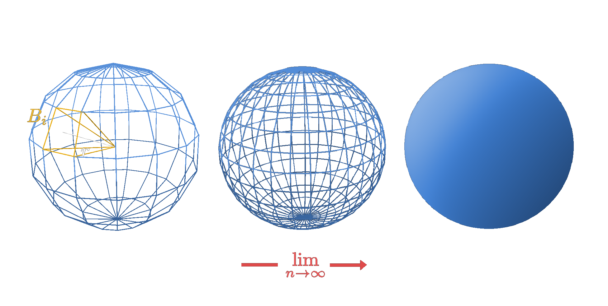
The volume of a cone is given by the area of its base \(B_i\) times its height, which in our case is the radius \(r\), divided by \(n\). The division by \(n\) might not be immediately obvious. While it is well-known in 3 dimensions that the volume of any kind of cone is the area of the base times the height divided by 3, it is less clear whether this extends to all dimensions. At least, for the 2-dimensional case, we see the division by \(n\) holds. Here, the cone reduces to a triangle, and the division by \(n\) is consistent. The area of a triangle is the base, which is the side length, times the height divided by 2. We will now explore how this principle can be proven for all dimensions.
Examining cross-sections of the cone at different heights reveals that each cross-section is simply a scaled-down version of the base area. Specifically, the scaling depends on how far we move from the base toward the top. Since each cross-section is an \(n-1\)-dimensional surface in an \(n\)-dimensional cone, the area of the cross-section scales with the proportion of the height we have moved up, raised to the power \(n-1\). For example, in the 3-dimensional case, if we move up to half the total height, the area of the cross-section will be \((\frac{1}{2})^2 = \frac{1}{4}\) of the base area.
This scaling down based on the ratio raised the power \(n-1\), directly follows from the definition of an \(n\)-dimensional cone. Take any planar \(n-1\)-dimensional shape as the base and draw a perpendicular line at its center. Then scale this shape linearly down along this line. The rate of it will determine how far you get, which defines the height of the cone. Needless to say, if the shape is scaled down linearly, the area will scale down by that rate raised to the power \(n-1\) because an area is always of one dimension less of measure by definition.
Summing things up and coming back to our concrete example of the cones that approximate a sphere (so the height of one cone is \(r\)), we can state the following
\begin{equation} V_n^{\text{cone}} = \int_0^r B (1-\frac{x}{r})^{n-1} dx, \end{equation}which just means we take the area \(B (1-\frac{x}{r})^{n-1}\) of each cross section and integrate it from the base up to the very top of the cone to get its total volume. Applying the substitution \(u=1-\frac{x}{r}\) to the integral leads to
\begin{equation} V_n^{\text{cone}} = - \int_1^0 B u^{n-1} du = - B \frac{u^n}{n}\bigg\rvert_0^1 \end{equation}which solves to the above stated formula of
\begin{equation} V_n^{\text{cone}} = B \frac{r}{n}. \end{equation}Deriving the surface area of an \(n\)-dimensional sphere
Having established these two facts about the surface and the volume will help us out tremendously in our attempt to solve for the surface area of a \(n\)-dimensional sphere. So let us move on to the actual derivation of the concrete formula that will provide us that surface area. As mentioned above, one possibility would be to figure out how a solution for lower dimensions scales as we scale the dimension \(n\). So, for instance, a recursion formula that tells us how to get from a formula for \(n\) to \(n+1\) will be just that. Let us try to figure out such a recursion rule.
Why is this approach of a recursion rule suitable in this context? Well, if we intersect any \(n\)-dimensional sphere with a hyperplane (a plane in an \(n\)-dimensional space), the cross-section will always be a sphere of \(n-1\) dimensions. If you do not see that at first glance, we will dig deeper into that in the following paragraphs. In the end, we will obtain the desired recursion formula by doing so.
First, let us put things into a geometric picture by using the familiar 3-dimensional space. Looking at the following illustration, we see a sphere that is intersected by a plane. The resulting cross-section is a circle, which is a 2-dimensional sphere.
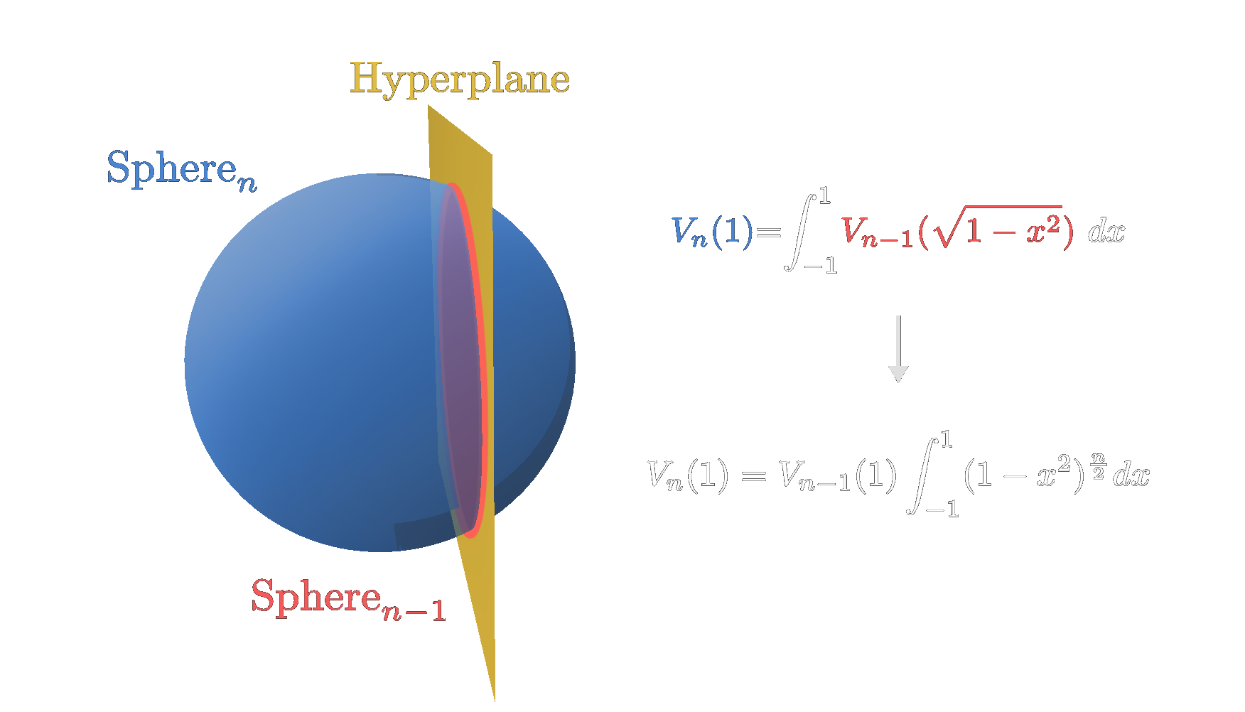
From the above figure, we can easily deduce that our conjecture holds for \(n=3\), however, what about the general case? Let us reason through more rigorously, leaving all the illustrations aside.
Let \(X_1,..,X_n \in \rm I\!R\) be arbitrary numbers and \(c_1, c_2 \in \rm I\!R:c_2^2 \leq c_1\) be fixed constants. If the set of all numbers, which satisfy \(\sum_{i=0}^n X_i^2 = c_1\) be called the surface of an \(n\)-dimensional sphere of radius \(\sqrt{c_1}\) and the set of all numbers \(X_j = c_2\) be called a hyperplane perpendicular to the j\(^{\text{th}}\) axes then numbers. What is the set of numbers that satisfy both conditions?
Well, for starters, limiting our analysis to a hyperplane perpendicular to a specific axis is sufficient due to the rotational symmetry of a sphere (This rotational symmetry for a set of numbers satisfying \(\sum_{i=0}^n X_i^2 = c_1\) can be proved easily by switching to spherical coordinates). Next, considering the condition \(\sum_{i=0}^n X_i^2 = c_1\) and the additional constraint \(X_j = c_2\), we get
\begin{equation} X_1^2+..+X_{i-1}^2+c_2^2+X_{i+1}^2+..+X_n^2 = c_1 \end{equation}which can be rearrange to
\begin{equation} X_1^2+..+X_{i-1}^2+X_{i+1}^2+..+X_n^2 = c_1-c_2^2 \end{equation}Obviously, if we choose \(c_3 = c_1-c_2^2\), it follows \(c_3 \in \rm I\!R\) and we are left with the same situation as in \(\sum_{i=0}^n X_i^2 = c_1\), just that we now sum up \(n-1\) terms and the constant is \(c_3\). Therefore we can call this new set of numbers a surface of an \(n-1\)-dimensional sphere with radius \(\sqrt{c_1-c_2^2}\). Needless to say, that would have also worked for the volume of a sphere, just replace the equal sign, with less or equal.
With this geometric insight established, we can now move on to establishing the recursion formula by finding the relationship between the cross-section of a \(n-1\)-dimensional sphere to the \(n\)-dimensional we obtained the cross section from. The most simple way is that we can just state, that the integral over all cross sections has to be again the volume of the original \(n\)-dimensional sphere, similar to how we did it with the cones that approximated a sphere. Doing that will lead us to
\begin{equation} V_n(1) = \int_{-1}^1V_{n-1}(\sqrt{1-x^2})dx. \end{equation}We can easily simplify this by using our first prerequisite of \(V_n(r)=V_n(1)r^n\), which changes the above equation to
\begin{equation} V_n(1) = V_{n-1}(1)\int_{-1}^1(1-x^2)^{\frac{n}{2}}dx. \end{equation}All we have to do now is to solve this integral. If you have any experience in calculus you will share the feeling that this integral is begging for a trigonometric substitution. After choosing \(x = cos(x)\) we are left with
\begin{equation} \int_{0}^{\pi}sin^n(x)dx. \end{equation}After making this substitution, the integral becomes much cleaner and simpler, but finding the final solution will still be challenging. To tackle this, we should use integration by parts. This method is particularly convenient when dealing with trigonometric functions in an integral because these functions recur in their derivatives and antiderivatives. Consequently, there is a good chance that trigonometric terms will cancel out, or, as in this case, that a recursive relationship can be established. Therefore, applying integration by parts leads to
\begin{equation} \int_{0}^{\pi}sin(x)^ndx = -sin^{n-2}(x)cos(x) \rvert_{0}^{\pi} \end{equation} \begin{equation} + \int_{0}^{\pi}(n-1)sin^{n-2}(x)cos^2(x)dx, \end{equation}whereby we see that the first term is actually just 0 and the second one can be expressed purely in terms of \(\sin\) functions
\begin{equation} \int_{0}^{\pi}sin(x)^ndx = \end{equation} \begin{equation} \int_{0}^{\pi}(n-1)sin^{n-2}(x)-(n-1)sin^n(x)dx, \end{equation}from which we are able to deduce the following recursive pattern
\begin{equation} I_n=\frac{n-1}{n}I_{n-2}, where \quad I_n = \int_{0}^{\pi}sin^n(x)dx. \end{equation}This again is sufficient to solve the integral because needless to say we know
\begin{equation} I_0 = \pi, I_1 = 2. \end{equation}This integral has also some importance outside of this context and it is possible to derive a converging product for \(\pi\) from it, the so-called Wallis Product. We will check it out in an upcoming Story.
Anyway, coming back to our context of an \(n\)-dimensional sphere, summarizing things, we can conclude that have found out
\begin{equation} V_n(1) = \frac{n-1}{n}\frac{n-3}{n-2}\cdots\pi\quad\cdot \frac{n-2}{n-1}\frac{n-4}{n-3}\cdots 2 \end{equation} \begin{equation} \cdot \frac{n-3}{n-2}\frac{n-5}{n-4}\cdots\pi \quad\cdot \cdots\cdot\frac{1}{2}\pi \cdot 2, \end{equation}whereby what the actual start term of this product is (either that one with \(\pi\) or the one with 2 at the end) depends on the fact if \(n\) is even or odd (In the above equation the case for \(n\) is even is shown exemplary). Nevertheless, it is obvious that lots of terms will cancel out each other. No matter if \(n\) is even or odd beginning with the first term the numerator will always cancel with the denominator of the following term, excluding the \(\pi\) terms and the 2's. Hence we are left with the denominator of the first term, which will be \(n (n-2) \cdots\) until 2 if \(n\) even or 1 if it is odd, and the numerator of the last term, which is just 1. The number of \(\pi's\) and 2's left, increases with every second step in \(n\)
\begin{equation} V_n(1) = \frac{\pi^{[n/2]} 2^{[\frac{n-1}{2}]}}{n(n-2)(n-4)\cdots} \end{equation}This result is quite promising, but the presence of Gaussian brackets and the distinction between even and odd \(n\) is somewhat unsettling. If we match the denominator, with the product of 2's in the numerator, we nearly obtain \(1 / (\frac{n}{2})!\) when \(n\) is even. For odd \(n\), we get a product of the form \(\frac{n}{2} \cdot (\frac{n}{2}-1) \cdot \cdots\). This sequence resembles a factorial sequence for half-integer values but does not perfectly interpolate the factorial sequence. Even if the concept of a \(\frac{3}{2}\)! factorial seems unconventional, we can agree that at least the property \((n-1)!n=n!\) should hold, which is satisfied by our product. Additionally, we could define \(\frac{1}{2}\) factorial to evaluate to a certain value such that it better interpolates the factorial numbers for whole integer values. Actually, \(\sqrt{\pi}\) would work perfectly for that and it additionally would also simplify the whole expression as it solves the inconvenience that the number of \(\pi\) terms is increasing every second step. Therefore, if we extend the factorial numbers in that way, both Gaussian brackets vanish and we are left with
\begin{equation} V_n(1) = \frac{\pi^{\frac{n}{2}}}{(\frac{n}{2})!}. \end{equation}Whether or not one interprets this function with the \(\sqrt{\pi}\) term as an extension of the factorial beyond natural numbers or not is ultimately a matter of perspective. It is certainly a reasonable extension of the factorial concept, but it can also be viewed as just a new function \(P\)
\begin{equation} P\Big(\frac{n}{2}\Big) = \Big(\frac{n}{2}\Big) ! \quad if \quad n \quad even, \end{equation} \begin{equation} \sqrt{\pi} \prod_{i=1}^{\frac{n-1}{2}} \frac{2i-1}{2i} \quad if \quad n \quad odd. \end{equation}which we have defined to make things cleaner and simpler. Indeed, it turns out that this function we have encountered (or extension of the factorials) recurs very often in mathematics and has been hence given a name, the gamma function, usually denoted as \(\Gamma(n)\). Its definition range covers the whole complex plane. However, thinking of the gamma function as merely the factorial for any complex number is as limited as believing \(\pi\) is just the ratio of a circle's circumference to its diameter. The gamma function is a far more difficult mathematical object to understand and one has to get to know different aspects of it, by encountering it over and over again, to finally arrive at a solid understanding of it.
Moving on with the equation for the volume of an \(n\)-dimensional unit sphere we have just obtained, we can easily extend it for the general case of any radius \(r\), by using our prerequisite from the very beginning, leading to
\begin{equation} V_n(r) = \frac{r^n\pi^{\frac{n}{2}}}{(\frac{n}{2})!}. \end{equation}Furthermore, we can also easily provide a formula for the surface by using the second prerequisite
\begin{equation} S_{n-1} = \frac{r^{n-1}n\pi^{\frac{n}{2}}}{(\frac{n}{2})!} = \frac{2r^{n-1}\pi^{\frac{n}{2}}}{(\frac{n}{2}-1)!} \end{equation}This allows us to finally complete the formula for the probability density function of our random variable \(Y\)
\begin{equation} Y_{PDF}(y)dy = (2\pi)^{-\frac{n}{2}}e^{-\frac{y}{2}} \frac{2y^{\frac{n-1}{2}}\pi^{\frac{n}{2}}}{(\frac{n}{2}-1)!} \frac{dy}{2y^{\frac{1}{2}}}. \end{equation}Obviously, the \(\pi\) terms and both terms of 2's will cancel and after summarizing the powers of y, we are left with
\begin{equation} Y_{PDF}(y)dy = e^{-\frac{y}{2}} \frac{y^{\frac{n}{2}-1}}{2^{\frac{n}{2}}(\frac{n}{2}-1)!} dy. \end{equation}And that is it. We have successfully found the probability density function for the random variable \(Y\). Rewriting our extended factorial function in terms of the gamma function and realizing that for negative numbers the probability is just zero (the considerations above only make sense if y is non-negative, cause a sphere with a negative radius does not make any sense), the final result is
\begin{equation} Y_{PDF}(y) = \left\{\begin{array}{ll} e^{-\frac{y}{2}} \frac{y^{\frac{n}{2}-1}}{2^{\frac{n}{2}}\Gamma(\frac{n}{2})} & \text{if} \quad x > 0 \\ 0 & \text{otherwise}\end{array}\right\} \end{equation}To conclude this derivation of the direct approach via the probability density function and the surface area of an \(n\)-dimensional sphere, let us look at a graphical plot of this PDF we have just found (We have now switch to the more familar notation \(f(x)\) instead of using \(y\) as the input variable, which is a little unconventional when talking about a function)
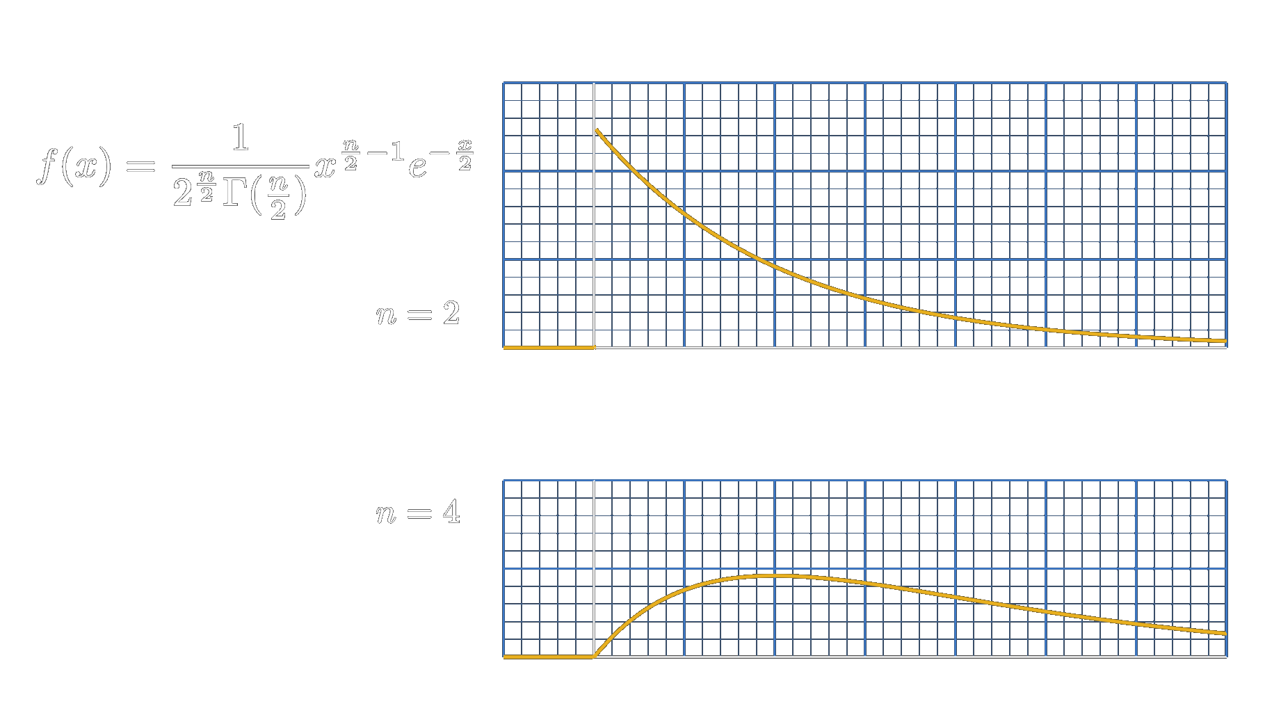
We observe that the shape of the graph changes significantly as \(n\) increases. For \(n=1\) and \(n=2\), the graph exhibits a steep, monotonically decreasing curve, as shown in the upper grid. However, for \(n=3\) and above, the graph transitions into a non-symmetric bell-shaped curve, with its peak shifting to the right as \(n\) increases. This behavior makes intuitive sense: as the number of squared terms in the sum increases, we expect the sum to yield a larger value, leading to this shift in the graph's maximum.
Geometric perspective on the cumulative distribution
For the sake of completeness, we will also take a glance at the derivation via the cumulative probability and then we will finally finish this Story off. We will keep things short as most of it is pretty similar to the approach we just discussed in detail above.
Starting at the very beginning, instead of asking for how often the sum tends to equal some specific \(y\) we consider
\begin{equation} P(Y\leq y) = P(X_1^2+..+X_n^2\leq y), \end{equation} whereby by putting this equation in the same geometric context leads again to a sphere. However, since we have \(\leq y\), we are not intereseted in the area of the surface of the \(n\)-dimensional sphere but we want to integrate over the whole space inside the sphere. Writing this integral out we get \begin{equation} \frac{1}{(2\pi)^{\frac{n}{2}}}\int_{x_i^2+..+x_n^2\leq\sqrt{y}} e^{-\frac{1}{2}\sum X_i^2}dx_1,..,dx_n. \end{equation}As already mentioned at the beginning, the main issue compared to the direct approach via the density is that \(e^{-\frac{1}{2}\sum X_i^2}\) is no longer constant with respect to the integral. Therefore, it will not be as easy as just computing the volume of an \(n\)-dimensional sphere. However, viewing this integral in spherical coordinates will ease things a little
\begin{equation} \frac{1}{(2\pi)^{\frac{n}{2}}}\int_{0}^{2\pi}\int_0^{\pi}..\int_0^{\pi}\int_0^{\sqrt{y}}e^{-\frac{r^2}{2}}r^{n-1}dr \end{equation} \begin{equation} \sin(\phi_1)^{n-2}d\phi_1\cdots\sin(\phi_{n-2})d\phi_{n-2}d\phi_{n-1}. \end{equation}We can obviously separate the individual integrals, leading to
\begin{equation} \frac{1}{(2\pi)^{\frac{n}{2}}}\int_0^{\sqrt{y}}e^{-\frac{r^2}{2}}r^{n-1}dr\int_{0}^{2\pi}d\phi_{n-1} \end{equation} \begin{equation} \int_0^{\pi}\sin(\phi_1)^{n-2}d\phi_1\cdots\int_0^{\pi}\sin(\phi_{n-2})d\phi_{n-2}, \end{equation}Here, we can easily see that the second integral evaluates to \(2\pi\). The other integrals, involving powers of \(\sin\), should look familiar: they are the same ones we encountered earlier when deriving the probability density function. As mentioned before, this integral is quite significant and appears frequently in various contexts, as you can now see for yourself.
Plugging in the \(2\pi\) term and the solution of the power of \(\sin\) integrals we derived in the previous section, we get
\begin{equation} \frac{1}{(2\pi)^{\frac{n}{2}-1}}\int_0^{\sqrt{y}}e^{-\frac{r^2}{2}}r^{n-1}dr\frac{(n-3)(n-5)\cdots}{(n-2)(n-4)\cdots}\text{ }\cdot \end{equation} \begin{equation} \pi\frac{(n-4)(n-6)\cdots}{(n-3)(n-5)\cdots}2\text{ }\cdot\text{ }\cdots \end{equation}Analog to before, beginning with the first term the denominator will cancel with the numerator of the following term, and the whole product can be reduced in a similar manner like in the previous section. The only difference is that this time we start at \(n-2\) and hence we are left with
\begin{equation} \frac{\pi^{[\frac{n-1}{2}]} 2^{[\frac{n-2}{2}]}}{(n-2)(n-4)\cdots}. \end{equation}Expanding the factorials in the same manner as before (or just defining a new function), the expression neatly simplifies to
\begin{equation} \frac{\pi^{\frac{n}{2}-1}}{(\frac{n}{2})!} \end{equation}Plugging this solution back into the collection of integrals from above, we can now state
\begin{equation} Y_{CDF}(y) = \frac{1}{2^{\frac{n}{2}-1}\Gamma(\frac{n}{2})}\int_0^{\sqrt{y}}e^{-\frac{r^2}{2}}r^{n-1}dr. \end{equation}The remaining integral may appear complicated, and indeed it does not have a solution in terms of elementary functions. However, if our goal is simply to obtain the PDF again, we do not actually need to solve it. By taking the derivative, the integral will effectively be eliminated
\begin{equation} Y_{CDF}(y)^{'} = Y_{PDF}(y)dy \end{equation} \begin{equation} = \frac{1}{2^{\frac{n}{2}-1}\Gamma(\frac{n}{2})}e^{-\frac{y}{2}}y^{\frac{n-1}{2}}\frac{1}{2\sqrt{y}}dy \end{equation} \begin{equation} = e^{-\frac{y}{2}} \frac{y^{\frac{n}{2}-1}}{2^{\frac{n}{2}}\Gamma(\frac{n}{2})}dy. \end{equation}As we can see, we match the result from the derivation via the density. We can see, that both approaches work perfectly fine, albeit the direct approach via the density is a little clearer because everything falls just neatly into its place such that all terms are actually constant and can be moved outside the integral.
But what about the cumulative distribution function? We stopped because we encountered an integral that had no solution in terms of elementary functions. However, it turns out that this integral is encountered quite frequently as well. The solution of the integral (to be exact a more general version \(\int_0^{x}e^{-t}t^{n-1}dt\)) is defined as a function, called the lower incomplete gamma function, usually denoted as \(\gamma(n,t)\). We will not go into any further details here, but using the so-defined function \(\gamma\) we can rewrite the cumulative distribution function of our random variable \(Y\) as
\begin{equation} Y_{CDF}(y) = \left\{\begin{array}{ll} \frac{1}{\Gamma(\frac{n}{2})}\gamma(\frac{n}{2},\text{ }\frac{y}{2}) & \text{if} \quad y > 0 \\ 0 & \text{otherwise}\end{array}\right\} \end{equation}If you are curious about how we arrive at this final formula, it is important to note that our extension of the factorial, the gamma function, is actually the solution to the integral \(\int_0^{\infty}e^{-t}t^{n-1}dt = \Gamma(n)\). This also explains why the integral up to \(x\) is called the lower incomplete gamma function, because it represents an incomplete integral, only integrating up to \(x\). Needless to say, there is also an upper incomplete gamma function, which starts at \(x\) and integrates all the way to \(\infty\). However, exploring the gamma function and its incomplete variations is beyond the scope of this Story.
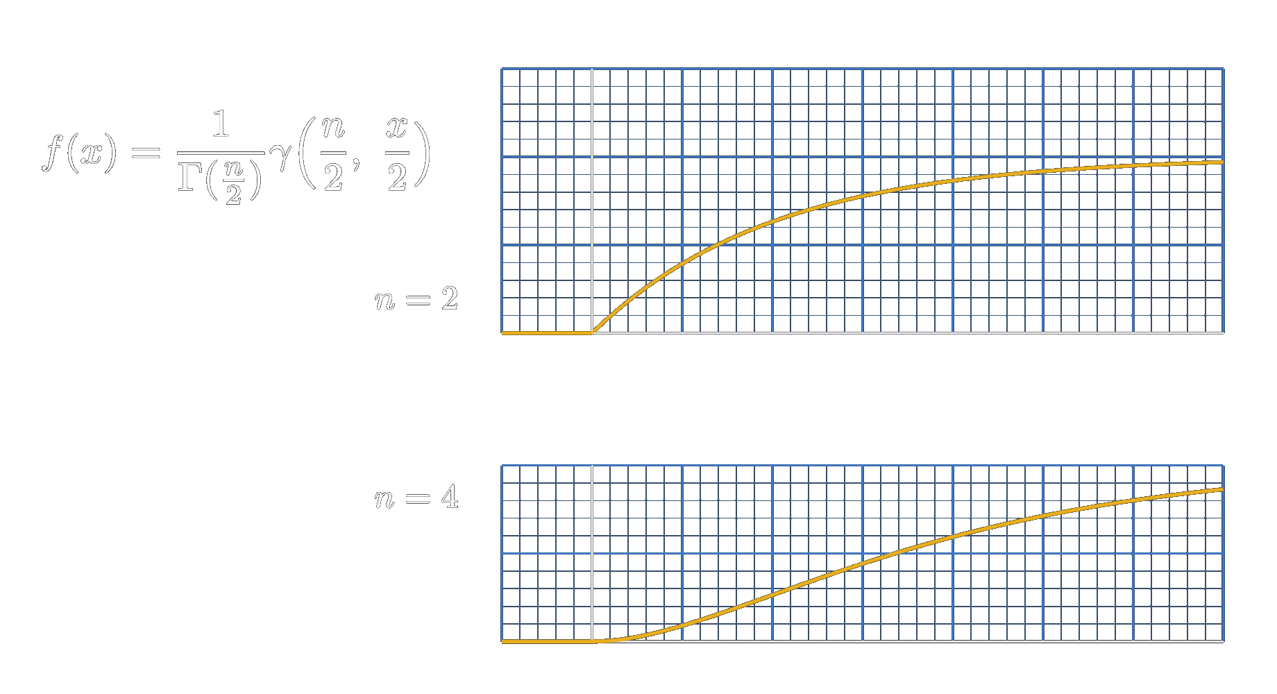
Instead, let us examine the cumulative distribution function we have just derived. In the figure above, the CDF is shown for \(n=2\) and \(n=4\), same as for to the PDF discussed earlier. As you can observe, for higher values of \(n\), the increase in cumulative probability becomes less sharp and more gradual.
Conclusion and outlook
That wraps it up for this story. We have successfully derived both the probability density function as well as the cumulative distribution function. For both, we started by putting the random variables involved into a geometric picture. Of course, such an approach always requires some higher degree of creativity but as we can see for most cases that is worth it as it often might simplify the problem. In our case, that meant we had just to solve for the volume and surface area of an \(n\)-dimensional sphere. That task on its own is needless to say quite heavy, however, it is a concrete isolated problem for which the solution for \(n\leq3\) is already known. Generalizing that solution to any arbitrary \(n\) finally led us to the solution of the PDF and CDF of our random variable \(Y\).
The so-derived distribution is usually referred to as the chi-squared distribution or \(\chi^2\) for short. It is the distribution of a sum of squared standard normally distributed random variables. Such a sum pops up quite frequently. Especially in the field of statistical tests, it is often possible to design the test quantity in such a way that it reduces to such a normalized sum.
As you might have already realized, the derivation of this distribution is rather cumbersome and lengthy. We have touched on a lot of different topics, like \(n\)-dimensional spheres or the various variations of the gamma function. We saw that both topics are heavily connected to the factorial numbers. Here we have just touched the tip of the iceberg and we certainly will dive deep into this connection in an upcoming Story but for now we will leave it at that.