Random variables
The concept of a random variable is a fundamental idea in probability theory. Although we will not delve into the precise definition and intricacies of this concept today, we will explore what happens when we apply a function to a random variable.
Consider, for instance, measuring a distance with a laser. The measured value will not be exactly the same each time, even if the laser is pointed at the same spot. This variability arises from environmental factors and imperfections in the laser measurement device. As a result, each measurement attempt yields slightly different values. Typically, these values follow a normal distribution around the true distance, which only an omniscient observer could know.
In practice, such measurements often serve as inputs for further computations and calculations. Naturally, the outcomes of these computations depend on the distribution of the input measurements. Therefore, it is advantageous to determine the distribution of the resulting values based on the input distribution. For instance, with this information, one can easily assess the precision of the computed values, which needless to say are of significant importance. Without an understanding of the variance or standard deviation, such computed values are often worth little to nothing.
Linear function of a normally distributed random variable
So let us proceed with a concrete derivation, using the familiar normal distribution and the simplest function we can think of: a linear function. Consider a random variable \(X\) that follows a normal distribution. We denote this as follows
\begin{equation} X \sim \mathcal{N}. \end{equation}Now, we apply a linear function to obtain a new random variable \(Y\)
\begin{equation} Y = aX + b, \quad Y \sim \text{ }?. \end{equation}Our goal now is to somehow find a way to determine the distribution of \(Y\).
First observation we can make, if we add a constant \(b\) that will obviously just shift the mean. Therefore, if \(aX\) follows a distribution \(\mathcal{D}\) then \(aX+b\) will follow the same distribution, just with an increased or decreased mean corresponding to the value of \(b\). Thus, the question essentially reduces to understanding the effect of multiplying a normally distributed random variable \(X\) by a constant.
A useful technique for solving such problems is to use cumulative probabilities. In our example, we can consider
\begin{equation} P(Y \leq y) \end{equation}whereby \(Y = cX\) with \(c \in \mathbb{R}\). Reformulating above probabilities leads to
\begin{equation} P(Y \leq y) = P(cX \leq y) = P(X \leq \frac{y}{c}) \end{equation}and since \(X \sim \mathcal{N}\) it follows that this cumulative distribution function (CDF) is given by
\begin{equation} Y_{CDF}(y) = \int_{-\infty}^{\frac{y}{c}} \frac{1}{\sqrt{2\pi\sigma^2}}e^{-(x-\mu)^2 / 2\sigma^2} dx \end{equation}There we have it, an expression for the cumulative distribution function of our random variable \(Y\). It's a rather complex integral, and it is difficult to deduce anything from it. So, let us try to find the probability density function as well. As you might know, the density function is just the derivative of the cumulative distribution function (if it is differentiable). Since this prerequisite definitely holds for our expression above, we can easily obtain the density by
\begin{equation} Y_{PDF} = Y_{CDF}' = \frac{1}{c}\frac{1}{\sqrt{2\pi\sigma^2}}e^{-(y/c-\mu)^2 / 2\sigma^2} \end{equation}This expression should look familiar; it is actually another normal distribution, just with a different variance (scaled by \(c^2\)) and different mean (scaled by \(c\)). If you do not see this immediately, try to factor out the \(c\) of the numerator in the exponent's fraction. This will lead to \(-(y-c\mu)^2 / 2\sigma^2c^2\). Then, after moving the division by c at the very beginning under the square root, you can see that
\begin{equation} \frac{1}{\sqrt{2\pi\sigma^2c^2}}e^{-(y-c\mu)^2 / 2\sigma^2c^2} = \mathcal{N}(c\mu,c^2\sigma^2). \end{equation}To sum things up, we have shown that a random variable \(Y=aX + b\), where \(X\) follows a normal distribution is again normally distributed. In particular if \(X \sim \mathcal{N}(\mu, \sigma^2)\) then \(Y\) is normally distributed with \(\mu = a\mu + b\) and \(\sigma^2 = a^2\sigma^2\) (taking also the already established fact that adding a constant \(b\) will just shift the mean of whichever distribution the original random variable had into account).
Importance of this result
The fact that any linear function of a normally distributed random variable yields again a variable that follows a normal distribution has quite significant implications. The normal distribution is undoubtedly the most common distribution when it comes to continuous probabilities. Due to the central limit theorem, a concept we will explore in another Story, the sum of random variables, no matter which distribution they follow, tends to converge towards the normal distribution.
Especially in real world applications, randomness and uncertainty is often caused by a sum of many smaller effects. Take for instance the example of the laser measurement device from above. The source of the hereby occurring random errors is rooted in many different things, like the temperature of the air the laser has to pass through, the properties of the surface the laser is reflected, some thermal noise in the measurement device and so on. This means the final small deviations from the true distance will be the sum of all those smaller errors, which consequently makes the normal distribution a very good approximation for the distribution of the overall error.
Furthermore, as the normal distribution is in most cases a good approximation for the underlying distribution of a random variable, a linear function is in most cases a good locally valid approximation for a function (around a given value). Such a function is the first degree Taylor approximation and it is given by the derivative of the function at this point. If the values do not deviate much from the Taylor point (the value for which the derivative has been calculated) the hereby obtained linear approximation will be very accurate.
What does this mean for the topic of applying functions to random variables? Well, it means there almost always exists a good approximation solution to such questions, no matter how complex the function actually might be. Given a random variable, if the variance is small enough (which in most real world applications will be the case) we can just compute the first degree Taylor expansion of the given function and we can easily determine the distribution of the resulting random variable. It will be given by \(\mathcal{N}(a\mu+b,a^2\sigma^2)\), whereby \(\mu\) and \(\sigma^2\) are the mean and the variance of the original random variable, respectively.
Needless to say, this is only valid locally, at the point of expansion of the first degree Taylor approximation. Additionally, we assumed a normal distribution, which might also not be correct. However, it is still the best approximation we can give, if nothing else is known about the distribution of the random variable and especially for most real world applications, where random errors are anyway often assumed to follow a normal curve, this approach is more than sufficient.
This method, known under the propagation of error, was originally introduced by Carl Friedrich Gauß. Up to this day, it is the most common way to determine the distribution and hence the variance and standard deviation of computation results yielded from values riddled with random errors.
Concrete example of using propagation of error
So let us work through a concrete example of using the method of propagation of error. Let us assume we have measured some angle \(\theta\) and we use this angle to determine the height of a building, as you can see in the following figure.
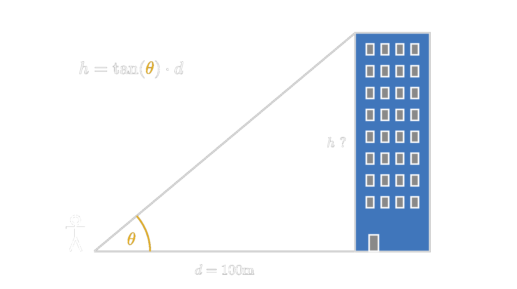
We have positioned ourselves a distance \(d\) of 100 meters away from the skyscraper for the measurement. Using the tangent function, we will be able to compute the exact height of it. However, since it is of course impossible to measure the angle completely accurate to the 100th digit after the comma, there will be some uncertainty involved. Some environmental factors, like shimmering air, could introduce even more variability.
Considering all those effects that influence our measurement, let us assume that we are able to determine the angle with a standard deviation of 0.1 degree. That means, we assume that our measurement we take will roughly be normally distributed with a standard deviation of 0.1 (i.e. \(\sigma = 0.01\)).
If we now calculate the height of the skyscraper, the question arises, how accurate is this result actually? So, what we are interested in, is the distribution of our resulting value if the input is distributed normally with \(\mathcal{N}(\theta, \sigma)\).
If we wanted to answer this question rigorously, we would have to determine the distribution of the result h, given by
\begin{equation} h = \tan(\theta) \cdot d, \quad \theta \sim \mathcal{N}, \end{equation}which needless to say is a rather cumbersome task to do. It could easily happen that this distribution is not expressible in terms of standard functions but we will only be able to provide a converging series. Luckily, however, we can use propagation of error, which will make this whole thing a walk in the park.
First, we have to find the best linear approximation for our function \(h = \tan(\theta) \cdot d\) at the point \(\theta_m\), which shall denote the actual measured value of \(\theta\). This is given by the Taylor polynomial of first degree, which leads to
\begin{equation} h_{linear}(\theta) = \tan(\theta_m) \cdot d + \frac{d}{\cos^2(\theta_m)} \cdot \theta. \end{equation}Now, we know that if we approximate our function with this linear function the resulting variable will be again normally distributed, whereby the mean is given by the original mean scaled by the slope of the linear function plus the constant from the linear function. The variance is given by the slope squared times the original variance. Applying this to our example results in
\begin{equation} \mu = \tan(\theta_m) \cdot d + \frac{d}{\cos^2(\theta_m)} \cdot \mu_{old} \end{equation} \begin{equation} \sigma = \frac{d^2}{\cos^4(\theta_m)} \cdot \sigma_{old}. \end{equation}Note that the equation for \(\mu\) is just the linear function evaluated for the input \(\mu_{old}\). Since \(\mu_{old}\) is actually unkown, the computation of \(\mu\) is reduced to just put in the obtained value \(\theta\) in the function. If we took several measurements, it would be possible to estimate \(\mu_{old}\), however there is usually not much to gain here. The variance, however, lets us deduce valuable infromation. For instance, if our measured angle is 41.5 degrees, the height evaluates to 88.47m, and we are now able to assess some information about the accuracy to this value. Namely, after plugging in the 41.5 degrees and a variance of 0.01 into above equation, we can state that the resulting height has a variance of 0.097, that means a standard deviation of about 0.31m. If we compute the result together with its variance for all possible \(\theta\), we see a clear trend. The higher the measured angle the less accurate is our computed height, as seen in the following image.
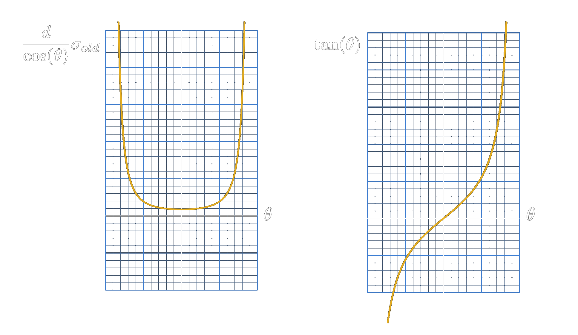
Let us see why this makes sense, by looking at both, the measurement setup and the involved tangent function. As can be deducted by looking at the graphical plot of the tangent function, the closer the values of the angle \(\theta\) get to 90 degrees, the more assymptotically the tangent function becomes. That means a very tiny portion of the \(x\)-axis is mapped to a huge area of the \(y\)-axis. Consequently, if there is some uncertainty in \(\theta\) the uncertainty in the height \(h\) gets blown up tremendously. The same holds if one imagines standing in front of a skyscraper and looking up to its very top. If you are very close, it does not matter if the building is 300 or 500 meters high, one would basically just look up straight, in an angle very close to the vertical. In constrast if one is positioned a kilometer away, the angle of sight is impacted quite drastically by the height of the building.
Raising normally distributed variable to the n-th power
Moving on with the topic of applying functions to a random variable, let us continue by elaborating yet another popular and rather simple function, the square function. In addition to, let us not limit to the power of 2 but try to generalize our findings and determine the distribution for all possible power functions (\(x^2, x^3, x^4, \cdots\)). For the distribution of the random variable, let us stick to the normal distribution.
We will again use cumulative probabilities and arrive at the density function by differentiation. Defining our new random variable by
\begin{equation} Y = X^n, \quad X \sim \mathcal{N} \end{equation}then we can state the following
\begin{equation} P(Y \leq y) = P(X^n) = \end{equation} \begin{equation} P(-\sqrt[n]{y} \leq X \leq \sqrt[n]{n}), \quad \text{if } n \text{ is even} \end{equation} \begin{equation} P(X \leq \sqrt[n]{y}), \quad \text{if } n \text{ is odd}. \end{equation}So we end up with two different cases, arising from the fact that even powers are guaranteed to cancel the sign of the input random variable, whereas odd powers do not. Computing the cumulative distribution function by integrating the density function of the random variable \(X\) for the cases leads to
\begin{equation} \int_{-\sqrt[n]{y}}^{-\sqrt[n]{y}} \frac{1}{\sqrt{2\pi\sigma^2}}e^{(x-\mu)^2/2\sigma^2} dx, \text{ } n \text{ even} \end{equation} \begin{equation} \int_{-\infty}^{-\sqrt[n]{y}} \frac{1}{\sqrt{2\pi\sigma^2}}e^{(x-\mu)^2/2\sigma^2} dx, \text{ } n \text{ odd}. \end{equation}We now need to differentiate both expressions. The first one is a bit tricky because both integral boundaries involve the variable \(y\), which is precisely what we want to differentiate. However, since the density of the normal distribution is perfectly symmetrical around 0, we can reformulate the integral by noting that it is twice the integral from 0 to \(y\). By doing this and differentiating, we obtain the following two density functions
\begin{equation} Y_{PDF} = \frac{2y^{\frac{1-n}{n}}}{n\sqrt{2\pi\sigma^2}} e^{-\frac{(y^{\frac{1}{n}-\mu})^2}{2\sigma^2}}, \text{ } n \text{ even}, \text{ } y \in \mathbb{R}^+ \end{equation} \begin{equation} \frac{y^{\frac{1-n}{n}}}{n\sqrt{2\pi\sigma^2}} e^{-\frac{(y^{\frac{1}{n}-\mu})^2}{2\sigma^2}}, \text{ } n \text{ odd}, \text{ } y \in \mathbb{R} \end{equation}As can be seen, the two probability densities are almost identical, differing only by a factor of 2. Let's examine a graphical plot of these two functions to better understand the difference.
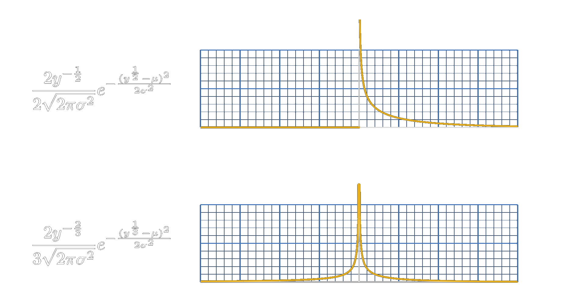
In the image above, the two densities are shown for \(n=2\) and \(n=3\). For even powers, the density for negative numbers is obviously zero. In the case of odd powers, we get a symmetrical graph. The overall shape of both densities is quite similar, peaking at \(x=0\) with a discontinuity and dropping towards zero as the absolute values of \(x\) increase. Why does this happen? Can we provide an intuitive explanation for it?
When raising a number to a power, two things can essentially happen: if its absolute value is less than one, it will decrease; if it is greater than one, it will increase. The number 1 represents a fixed point, where no matter which power we choose, the result will always remain at 1. Using this fact, how can we explain the drastic drop in the density as we move away from zero?
Let us consider an arbitrary interval that lies entirely within the 0 to 1 range. If we ask which points will fall into that area after raising our variable to some power, we can make a few observations. First, we know that the original area must lie slightly to the right, meaning it contains larger numbers. Why? Because in the 0 to 1 range, numbers get smaller when raised to a power. Second, the area must also lie completely within the 0 to 1 range. Why? Because if it didn't, applying the power function would map the area to a region which is at least partly greater than 1, contradicting our assumption that the interval lies fully within the 0 to 1 range. Third, we know that this area must be larger than the one after the power function has been applied. Why? Because the derivative of a power function is strictly less than one in the interval from 0 to 1.
What does this all mean? This implies that any interval in the 0 to 1 range gets condensed into a smaller one, lying even closer to zero than the original one when a power function is applied. Needless to say, this implies that the likelihood of the random variable will increase around 0.
Furthermore, if we take a look at the other range, the greater than 1 range, exactly the opposite is true. Every interval gets spread out and gets mapped to a wider interval even further away from 1 than the original one. Consequently, the likelihood of the random variable will decrease and the density function will have smaller values there.
These considerations make particular sense if we start from a uniform distribution. If the distribution of the random variable had a very low density around 0, this might offset the effect. However, in our case, the normal distribution already has a higher density near zero, so this effect is even amplified, resulting in an extremely sharp drop in the density as the values on the \(x\)-axis increase. Obviously, the higher the power to which we raise our random variable, the sharper this drop-off becomes (Because the derivative becomes significantly less in the range from 0 to 1 and substantially higher for values greater than 1 if the power is increased, the effect of condensing or spreading out gets even more pronounced than it is for lower powers.).
Different techniques for determining the distribution
We have now gone through two examples: firstly, a linear function and secondly, power functions, both with the random variable constrained to follow a normal distribution. The technique of rearranging cumulative probabilities worked well for these examples. However, are there cases where this approach fails? And what about distributions other than the normal distribution?
Generally speaking, the approach via cumulative propabilities does basically always work. However, it can get tricky, becuase we have to find \(P(X \leq \cdots)\). This was straightforward for a linear function and relatively simple for odd powers. However, for even powers, it became more challenging. We relied on the symmetry of the normal distribution around zero, which is necessary because even powers are non-monotonic functions.
Let us delve deeper into this by generalizing the approach through cumulative probabilities. Consider a random variable \(x\) following a distribution \(\mathcal{D}\). Now, let's apply a function \(f\) to it, yielding a new random variable
\begin{equation} Y = f(x), \text{ } \sim \mathcal{D}. \end{equation}Then let us consider the cumulative probability \(P(Y \leq y)\), which can be rearrange to
\begin{equation} P(Y \leq y) = P(f(X) \leq y). \end{equation}In the next step, we always isolated \(X\), since this is the variable we started with and we know its probability density function. This allowed us to easily integrate up to the expression on the right side of the inequality, giving us a formula for the cumulative distribution function of \(Y\). To isolate \(X\), we simply need to determine the inverse function of \(f\), which leads to
\begin{equation} P(Y \leq y) = P(f(X) \leq y) = \end{equation} \begin{equation} P(X \leq f^{-1}(y)) = \int_{-\infty}^{f^{-1}(y)} \mathcal{D}(x) dx. \end{equation}However, what if this inverse function \(f^{-1}\) does not exists? In that case, you need to split the function \(f\) into sections for which an inverse does exist and compute those cases separately (if two sections map to the same range of \(Y\) you have to take the sum). This is what we did, for instance, with the even powers in the example of the power function applied to a normally distributed random variable. We handled the set of negative and positive numbers separately, and since both map to the range of all positive numbers on the \(y\)-axis, we summed the two results. In our case this summation effectively evaluated to just multiplying the integral by two.
For now, to not complicate things and arrive at a general solution for the cumulative probabilities approach, let us continue with the assumption that a global valid inverse function exists which means we have to add the requirement that \(f\) is strictly monotonic.
Assuming that, we can move on to determining the density of \(Y\) by differentiating the above integral expression with respect to \(y\). The derivative of the integral will be given by
\begin{equation} PDF_Y(y) = D(f^{-1}(y))f^{-1}\text{ }'(y) \end{equation}This final expression is usually referred to as the change-of-variable technique, as it is the standard solution to solve for the distributions when applying functions to random variables. Essentially, it is the formal generalized result of our approach via the cumulative probabilities. However, despite its generalized character, there are some limitations to this technique, as you already have seen. For example, if the inverse of \(f\) does not exist, it becomes problematic. Additionally, \(f\) must be differentiable (everywhere except on a finite set of points, to be precise). While this approach can be cumbersome, the expression above is essentially what you need to solve to determine the distribution of the new random variable. You might find some geometric tricks or similar methods to solve for certain distributions, but they all basically solve the above equation, albeit in a very creative way.
As conclusion let us look what such a creative geometric technique could look like. Consider a set of \(n\) random variables \([X_1, \cdots, X_n]\). Let us define a new random variable by
\begin{equation} Y = X_1^2 + \cdots + X_n^2. \end{equation}As you can deduce from the equation above, we are dealing with a multidimensional problem, where we have \(n\) random variables as inputs to our function, which maps them to the new random variable \(Y\). We will not delve into the specifics of why this particular function might be of interest, but it is, nevertheless, a function applied to random variables. Therefore, this is a problem that one might encounter.
Tackling it with the standard technique of change-of-variable leads to
\begin{equation} P(Y \leq y) = P(X_1^2 + \cdots + X_n^2 \leq y). \end{equation}The next step would be to isolate all the \(X\), which is not really possible. However, there is an easy shortcut if we put things into a geomtric picture. Let us imagine a coordinate axis for each random variable \(X_i\) representing all the possible values this variable can take on. All \(n\) random variables together define a \(n\)-dimensional coordinate system. What does \(P(Y \leq y)\) asks for in this geometric setting?
Since \(Y = X_1^2 + \cdots + X_n^2\), asking for the values of \(X_i\) such that \(Y\) is less than or equal to some given number \(y\) essentially defines a \(n\)-dimensional sphere with radius \(\sqrt{y}\) in this coordinate system . All the points \([x_1,\cdots,x_n]\) that lie within this sphere will evaluate to a number \(\leq y\). This is a pretty good insight, right? Because now finding the cumulative propability \(P(Y \leq y)\) reduces to integrating the desnity of all \(X_i\) over this sphere. Finally, we then need to just differentiate the resulting integral expression and we have already obtained the PDF of \(Y\).
The detailed derivation of this PDF, however, requires finding a formula for the volume of an \(n\)-dimensional sphere, which eventually leads to the Gamma function. So there is still quite a lot of work to do. We will hence omit the details here, but if you are interested in this derivation, you can check out this Story.
As a final point, we will investigate an approach that is quite drastically different from the ones we have discussed before. This technique, known as the technique of moment generating functions, approaches the problem from a completely different perspective.
We will not delve into the details of a moment generating function here, but if you are interested, you can explore this Story. Assuming familiarity with the topic, if we have, for example
\begin{equation} Y = aX + b, \text{ } X \sim \mathcal{D} \end{equation}then we can obtain the density function of \(Y\) by firstly determining the moment generating function of \(\mathcal{D}\), which we will call \(M_X\). Then we can apply the above defined function to the moment generating function, which in our case is a linear function for which the result is well known and hence the moment generating function of \(Y\) will be given by
\begin{equation} M_Y(t) = e^{bt}M_X(at). \end{equation}Finally, all that is left is to retrieve the density function from the just derived moment generating function. Depending on the original distribution \(\mathcal{D}\), this task can be quite straightforward, allowing for a relatively easy solution for the distribution of \(Y\) using this technique. However, whether this technique is applicable in the first place depends of course on the specific details of the problem at hand.
Conclusion and outlook
In this exploration of random variables and the application of functions to them, we've covered several key concepts and derived important results. The primary takeaway is that applying a linear function to a normally distributed random variable yields another normally distributed variable. This result, rooted in the properties of normal distributions and linear transformations, has profound implications for various practical applications, especially in the context of error propagation.
Regarding other distributions and function we dipped our toes in the water a bit, but there are still million things left to explore. What is especially interesting are those problems where standard approaches do not work and one has to get creative like we saw in the sum of squared variables example. So, to conclude, the study of random variables and their transformations is a rich field with significant theoretical and practical implications - and in upcoming Stories we will take a look at the most exciting aspects of those. Stay tuned for new inspring Stories ahead!